TFA -
Time frequency analysis
and
-modification
Software package: Version 2.033, 30.07.10
This documentation: 30.07.10

IND - Ingenieurbüro für Nachrichten- und Datentechnik
Dr.-Ing. Peer Dahl
Keplerstrasse 44
D-75175
Tel. 49-7231-650332
Fax: 49-7231-965186
eMail: P.Dahl@ind-technik.de
Internet: www.ind-technik.de
Preface
Honored customer,
honored user!
Many thanks, that you decided
for this software product worldwide unique according to current research for
the purpose of the time frequency analysis. As you certainly know, the special
thing of this program lies in the contained algorithms (calculation methods)
for the breakup of the general attachment between time and frequency
resolution, which seen physical is regarded as impossible up to now.
The today available
processing power allows both the development and then the use of algorithms,
which denote a significant progress here. These flowed into TFA
directly.
For interested: Some time-frequency
analysis theory – what’s it all about?
To gain deeper insight into
the frequency characteristic of signals the Discrete Fourier transform (DFT)
today surely is one of the most frequent and in all fields of Digital Signal Processing
used analytical tools. The spectral description of a process can in addition be
starting point for purposeful manipulations in the frequency domain as a useful
alternative to the processing in the time domain.
Phenomena to be examined in
practice are frequently of instationary nature and are available only for a
restricted time interval. Although the DFT is defined unlike the time-discrete
Fourier transform only for a temporary process, the measurement period,
necessary to obtain a certain frequency accuracy, can be still considerably too
large. Meanwhile in case of instationary processes the minimization of the measurement
period is to strive also for obtaining a satisfactory temporal localization of
the result. Under these conditions the DFT supplies only a more or less
indistinct estimate of the context.
Since Werner Heisenberg
formulated his famous uncertainty relation of the quantum mechanics in the year
1927, also its analogy in the communication engineering therefore remained of
special importance until today.
Its consequence for the
spectrum analysis is that the priority between achieved frequency accuracy on
the one hand and the temporal localization on the other hand is to be decided
on. Both information can not be given simultaneously “exactly”. If a spectrum
shall represent only a short time interval, a coarse frequency resolution is to
be reckoned. If one increases the requirement onto the frequency resolution,
this requires a correspondingly longer analysis time interval. The fundamental
relationship between these two terms can be numerated exactly and comprehended
with every spectrum analyzer - whichever the principle of operation is.
On on hand one became accustomed to this association today, on the other
hand the restrictions turning out are so serious that until today worldwide endeavour
is made to searched for new ways out. It is to be observed that solutions known
up to now
· show disturbing
side effects due to non-linearities as occurrence of cross products and phantom
signals that do not exist (e.g. in case of the Wigner-Ville approach),
· do not meet the claim
by a more precise consideration (e.g. in case of the Wavelet-transformation),
· to presuppose unrealistic
conditions (e.g. the use of Gabor coefficients) or
· require Apriori-knowledge
(e.g. Linear Predictive Coding, LPC)
and therefore their use is
possible only for selected fields of application.
TFA contains a new
solution, which does not have the known disadvantages or in decisively smaller
extent.
Now we wish you a lot of
success and new analysis epertise about your signals which never before were to
be achieved in this quality.
Yours
IND - Ingenieurbüro für Nachrichten- und Datentechnik
Dr.-Ing. Peer Dahl
Keplerstrasse 44
D-75175 Pforzheim
Tel. 49-7231-650332
Fax: 49-7231-965186
eMail: P.Dahl@ind-technik.de
Internet:
www.ind-technik.de
Inhalt
2 System requirements, installation
and deinstallation
2.2.2 For less practiced users
4.1 The work space with the
representations time domain, frequency domain and time-frequency domain
4.1.1 The representation „Time domain“
4.1.2 The representation „Frequency
domain“
4.1.3 The representation „Time-frequency
domain “
4.1.4 Selection and sizes of the
representations
4.2.1.1.1 WAV-Format, 16 Bit, 1 channel (mono)
4.2.1.1.2 WAV-Format, 16 Bit, 2 channell (complex)
4.2.1.1.3 WAV-Format, PCM, 24 Bit and 32 Bit, 1 channel and 2 channels
4.2.1.1.4 WAV-Format, FLOAT, 32 Bit, 1 Kanal
bzw. 2 Kanäle
4.2.1.1.5 TFA-Format, 32 Bit, 1 channel (real)
4.2.1.1.6 TFA-Format, 32 Bit, 2 channel (complex)
4.2.1.1.7 TXT-Format, Textfile
4.2.1.2 Export (complex) respectively Export (real)
4.2.3.1.1 Level-Colour-Assiociation
4.3.4 Presentation continuous /
discrete
4.3.10 Vertikal harmonic marker
4.3.11 Horizontal harmonic marker
4.3.12 Advanced XY-Marker functions
4.3.14 Advanced zoom/boundary functions
4.3.15 Spectrum analysis settings
4.3.15.6 Further explanation of the
settings
4.3.16.6 Lower level threshold
4.3.17 DDC – Digital Down Converter
4.3.17.4 Automatic setting of the DDC
5.1.1 Speech signal: F0-analysis in
natural language
5.1.2 Communication engineering:
FSK-signal with shift- and modulation rate measurement
5.2.1 Speech signal: Extraction of the
F0-oscillation
5.2.2 Communication engineering:
Extraction of a FSK-signal
5.3.1 Speech signal: Making audible a
discant voice component
5.3.2 Communication engineering:
Conversion of a real-valued signal into the complex base band
5.3.2.2 New TFA instance with DDC-result
5.4 Analysis of Modulation spectra
5.4.1 Selection and extraction of a
frequency component as its envelope
5.4.2 Analysis of the modulation spectrum
6 FAQ – Frequenzly asked questions
6.1 Uncoupling XY-Marker and mouse
pointer
6.2 Long duration of DXP-I-computation
6.4 Unsatisfactory spectral resolution
6.5 Staircase-shaped time signal after
DDC-decimation
6.6 Installation on a network drive
9.1 Layout of the TFA-File-Format
TFA
–
Time frequency analysis and
-modification
1
General
Primarily the software product TFA is used for time-frequency
analysis, that means the simultaneous description of a signal both in
direction of the time axis as also the frequency axis. That shows a
tridimensional representation, the spectrogram, at which the signal
energy is colored as a third dimension characterized (e.g. high energy: red,
low energy: blue to black). If the signal sample to be analyzed is something
audible, one mentions the spectrogram also „sonagram”.
Whether signals, however, come from the world of audible, whether they
represent physical or other scientific processes, or whether they are signals
from the sundry communication engineering, e.g. the digital radio, is
unimportant: In all cases conventional spectrographs can represent the time-frequency
domain only with the typical uncertainty according to Heisenberg’s
uncertainty relationship of communication engineering.
An example to that: In the following a speech sample[1] is analyzed with
a conventional Hann-windowed fast Fourier transform (FFT) with a length of
4096:
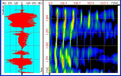
Figure 1‑1: Speech sample, transformation
FFT, FFT-length 4096
That offers a quite precise resolution into frequency direction (3,91
Hz), however, a
coarse temporal resolution (about 0,256 s). The speech pauses are very
blurredly represented.
The temporal resolution can be increased through decrease of the
FFT-length onto the value 512 by the factor 8 as following spectrogram shows.
That offers a correspondingly coarse resolution in frequency direction (31,25
Hz), for that, however, a more precise temporal resolution (about 0,032 s). Now
for example the speech pauses are more precisely represented.
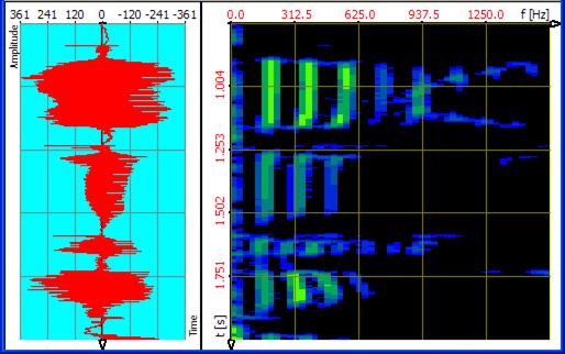
Figure 1‑2: Speech sample, transformation FFT, FFT-length 512
With TFA the signal can be exactly surveyed both in frequency-
and also in time direction. That performs the new transformation method DXP-I
eligible instead of the FFT. With DXP the frequency resolution (up to 4096
lines) and the time interval coming in (e.g. 512 samples) can be adjusted
separately from each other as following spectrogram shows. In a way one obtains the best
from the two above representations:
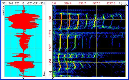
Figure 1‑3: Speech sample, transformation DXP-I, FFT-length 4096, 512 samples
Also a considerably more precise energy measurement is accompanied by
the significantly sharper representation of the time-frequency domain because
the signal energy is not distributed so very much in the plain anymore.
Based on a more precise spectrogram also the signal modification is possible in the time-frequency domain with higher
quality. As described later, eligible areas can be extracted in the spectrogram
or can be time-/frequency-agile filtered.
Important notice:
TFA and DXP are new, still little spread tools, that are not - that
is preceded - difficult to master. However, a little bit of practice and also
knowledge and experience is useful in order to be able to draw the full benefit
from that. Who is not yet so familiar to DXP, the short chapter 5 “practices” is warmly recommended to. It offers an introduction
and is considered as a starting point for the exploration of the own signal
material.
2
System
requirements, installation and deinstallation
In this section you find out,
how the software TFA is put into- and removed from operation.
2.1
System requirements
The least system requirements
are:
- Operation system: Windows
XP (SP2) Windows Vista or Windows 7
- Internet-browser for the display of help-files
- Main memory: 512 MBS
- Hard disk place: 20 MByte
- Processor clock: 2 GHz
- 1 free USB port for the dongle (copying
protection stick)
TFA manages also with
smaller resources, nevertheless: The higher the processor clock is, the shorter
the program reaction times are, especially in the case of the
DXP-transformations. A bigger main memory facilitates the enlargement of the
program windows onto the faces of two monitors (dual monitoring mode) also in
case of high screen resolution from 1280 x 1024 pixels. A bigger main memory
also facilitates the operation with very large signal files.
Recommended is:
- Double core processor system (Dual-Core, Core
Duo) with 2x3 GHz clock frequency
- 1 or 2 GB main memory
- Graphic with high resolution (1280 x 1024)
Even if TFA can
currently only use one processor, in case of a multiprocessor system it is nevertheless
possible to start a second instance of TFA in parallel and independently
of each other. In addition the operating system reacts to other inputs more
quickly, because TFA does not “block” the system.
2.2
Installation
TFA is - how many
other
TFA is delivered as a
ZIP-archive. The ZIP-archive contains the folder „TFA", under that all
needed subdirectories and files lie.
For the installation the
ZIP-archive is to be unpacked into an arbitrary folder. To do this one extracts
the complete folder „TFA" including its subdirectories and files onto an
arbitrary place on the hard disk.
Notice: You must have
administrator-rights!
2.2.1
For expert users
Please copy the contents of
the ZIP archive under retention of the directory structure onto an arbitrary
place of your hard disk and plug in the USB dongle into a free USB port.
2.2.2
For less practiced users
Maybe you wish to save the
„TFA"-folders in a new subdirectory e.g. with the name „TimeFrequencyAnalysis".
Please proceed then in following steps:
Step 1: Creation of a
folder named „TimeFrequencyAnalysis " on the hard disk.
To
that
- one opens the Windows-Explorer e.g. with the key
combination „<Windows> + <E>",
- choose a folder on the wanted hard disk drive or
create one at a wanted folder place by pressing of the right mouse button,
then ->New->Folder. Now one enters e.g. „TimeFrequencyAnalysis
" and confirms that with the „return" –Key.
Step 2: Unpack the ZIP
archive into the before created folder. According to that, as you acquired the
TFA-ZIP archive,
- it is stored on a storage medium or
- lies as download e.g. in your download folder or
- is managed by your download-manager-software.
Please open the ZIP-archive
with a double-click with the left mouse button onto the ZIP-file or by clicking
onto the key „Proceed" (or comparably similar) in your download-manager.
The indicated contents of the
ZIP-archive are to be copied with the right mouse button and to be pasted into
the folder created in step 1.
Possibly you would like to
create further folders in the folder „TimeFrequencyAnalysis" e.g. for your
signal files. In this case your directory structure looks e.g. as follows:
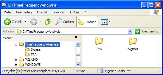
Figure 2‑1: Possible directory structure for the program installation
Step 3: Plug in the
Dongle „TFA" into a free USB port.
Tip: The best choice is a
USB-port on the back of the computer so that a mechanical harm of the Dongle
and the computer while pushing inadvertent is avoided.
No automatic installations
occur while plugging in the Dongle
2.3
Installation of updates
Please simply copy new files
into the TFA-folder and hereby overwrite older files with the same name.
2.4
Deinstallation
The complete deinstallation
is simple: To that
- one opens the Windows-Explorer e.g. with the key
combination „<Windows> + <E>",
- chooses the folder into which the installation was
performed,
- clicks with the right mouse button on it and
chooses the command “delete".
3
Start of program
The program is started by a
double-click with the left mouse button onto the file „TFA.exe". To that one
- opens the Windows-Explorer e.g. with the key
combination „<Windows> + <E>",
- selects the folder into which the installation
was performed,
- carries out a double-click with the left mouse
button on the file „TFA.exe ".
Notices for more convenience:
More convenient may be the
one-time setup of a link on the desktop. To this one
- opens the Windows-Explorer e.g. with the key
combination „<Windows> + <E>",
- selects the folder into which the installation
was performed,
- performs a right-click on the file „TFA.exe"
and chooses „create link” (or comparable).
- The new linking may then be pulled onto the
desktop with left mouse button.
Instead of the creation of a
linking one can stitch „TFA.exe" also onto the start menu. To that one
- opens the Windows-Explorer e.g. with the key
combination „<Windows> + <E>",
- selects the folder into which the installation
was performed,
- performs a right-click on the file „TFA.exe"
and choosees and „stitch to start menu” (or comparable).
One notices, however, that in case of a
deinstallation the convenience-steps are to be revoked manually (deleting
desktop-linking and/or to deleting program from start menu).
4
The TFA progam window
When starting the program the following program window is shown
according to the chosen view-options:
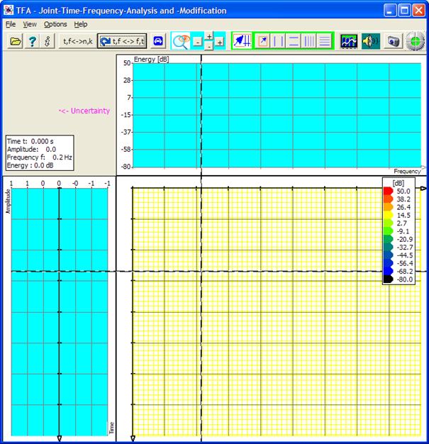
Figure 4‑1: The TFA programm window after program start
Opening e.g. the WAV-file „IND_TFA.Wav" (contained in scope of
delivery) with the command “open file”, one already obtains an analysis with
the representations of time domain (to the left or above), frequency domain
(above and/or to the left) and the time-frequency domain (to the right -
below):
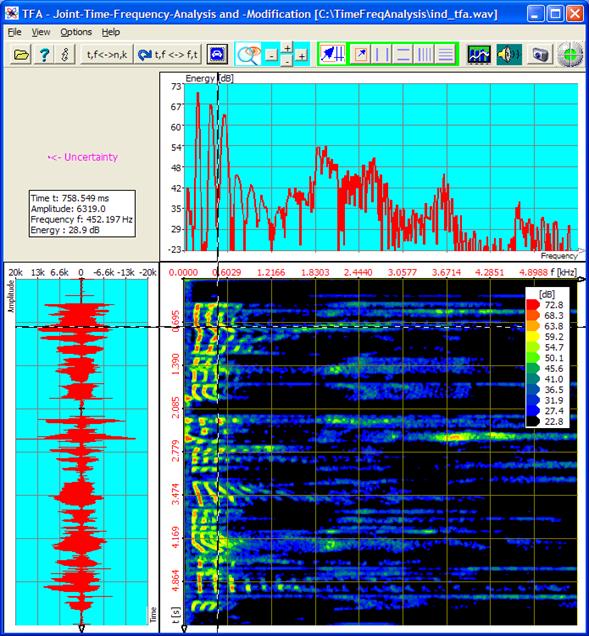
Figure 4‑2: TFA after opening file „IND_TFA.Wav“, FFT-lenght:
1024
As with most Windows-programs there is:
·
The menu bar
·
Short-Keys for frequently used functions and commands
·
The work space, that contains the three
representations time domain, frequency domain and time-frequency domain
·
Next to that some measurement tools are to be seen
according to the chosen options.
These program elements shall be explained now. The beginning does „The
work space with the representations time domain, frequency domain and time-frequency
domain”, because it allocates the biggest area in the main window.
4.1
The
work space with the representations time domain, frequency domain and time-frequency
domain
The figure above shows already
the most important elements of the work space, the three representations:
- Time domain
- Frequency domain
and
- Time-frequency
domain
4.1.1
The representation „Time domain“
It corresponds to an oscillogram of a time signal. Its axes are
correspondingly scaled with „time” and „amplitude". This representation
type is included in many products for signal analysis and does not contain any
special features. The graphic can be arranged to the left, as shown in the
figure above, or arranged in the upper working area, cf. section 4.3.5.
4.1.2
The representation „Frequency domain“
This representation shows the
spectrum of the time interval, whose centre corresponds to the temporal
coordinate of the mouse pointer in the time-frequency representation, see
below. The transformation parameters, therefore
- transformation
method
- spectral- and temporal resolution
- window functions
are explained in section 4.3.15 „Spektralanalysis settings„. The graphic can be arranged upside, as shown in the
figure above, or in the left of the work space, cf. section 4.3.5.
4.1.3
The
representation „Time-frequency domain “
One can imagine this
representation, known also as a spectrogram or in case of voice signals
as sonagramm, as a common view of the frequency domain representations
of all shown points in time, and that in a single graphic. The in this
way necessary third coordinate could be obtained by changeover from the
two-dimensional to a cube. However experiments show, that shadowing effects may
hide signal components easily.
Most superior is the coloured
presentation of the third coordinate to which the energy is assigned. The way
energy and colour are associated is handled in section 4.2.2.4.
The graphic is always placed
below/to the left in the work space, however, the axis meaning conforms to the
arrangement of the other two graphics because bordering axes are common.
Usefull
note:
A double-mouse-click in this
representation initiates the storage of the spectral line vector (dB-scaled,
txt-format) for the point of time according to the mouse position. The
localization of the txt-file is the TFA
working dircectory. Point of time and the frequency resolution form the file
name.
4.1.4
Selection
and sizes of the representations
In Figure 4-2 a proposal for the sizes of the three representations
is given. For the benefit of a certain representation it may be sometimes
better to draw a graphic in a smaller way or completely to renounce it.
That is simply possible
through mouse-drawing of the window boundaries. As soon as the mouse pointer is
in the area of a window boundary, the typical mouse pointer symbol indicates
the readiness to size the figure. The following two figures give examples:
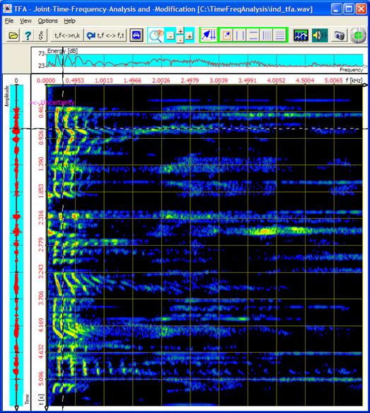
Figure 4‑3: TFA with enlarged time-frequency representation
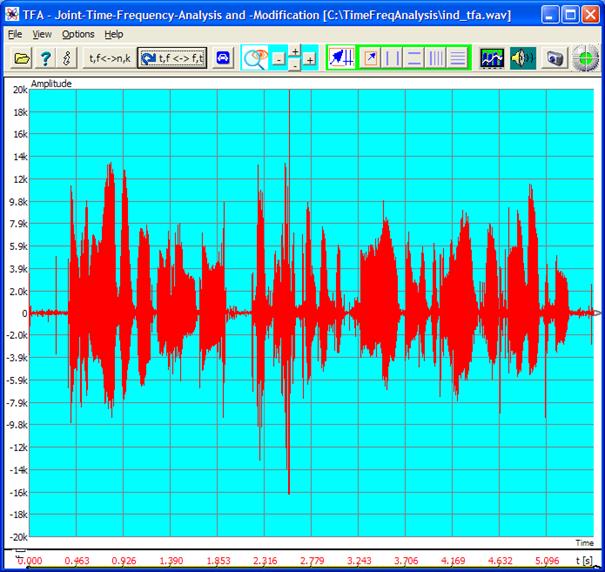
Figure 4‑4: TFA with enlarged time representation
4.2
The
menu bar
![]()
The menu bar includes the points
- File
- View
- Options
- Help
The next sections pay attention to them.
4.2.1
File
It is selectable:
- Open…
- Export
- Close
4.2.1.1 Open
TFA can handle six file formats:
- WAV-Format,
16 Bit PCM, 1 channel (mono) und 2 channel (complex)
- WAV-Format,
24 Bit PCM, 1 channel (mono) und 2 channel (complex)
- WAV-Format,
32 Bit PCM, 1 Kanal (mono) und 2 channel (complex)
- WAV-Format,
32 Bit FLOAT, 1 channel (mono) und 2 channel (complex)
- TFA-Format, 32 Bit, 1 Kanal (mono,
reell-wertig) und 2 channel
(complex)
- TXT-Format, Textfile
4.2.1.1.1 WAV-Format, 16 Bit, 1 channel (mono)
PCM-16-Bit is the mostly used
format. Normally a signal recording will subsist as a one-channel real valued
file, therefore a usual recording in mono.
4.2.1.1.2 WAV-Format, 16 Bit, 2 channell (complex)
TFA can also handle
complex valued signal files. Such can arise e.g. at the output of a digital
down converter (DDC) and contain a real part (Re) and an imaginary part (Im).
The sample sequence within the file is (Re), (Im), (Re), (Im).... . For this
two-channel file format the use of the Stereo-WAV-format has prevailed. Instead
of the left-/right-Information the two channels are interpreted as real part
and imaginary part. TFA cannot be
used for processing stereo files.
Notice: In order to be
able to process this file format still more precisely, at first a sampling rate
doubling is performed in TFA. Through that the measurement properties
improve, but the indicated sample numbers have the double valuation in the
comparison with the file. Time and frequency reference is not affected by that
of course.
4.2.1.1.3 WAV-Format, PCM, 24 Bit and 32 Bit,
1 channel and 2 channels
These formats are similar to
those described in the two sections before. The difference is the use of 3 and
4 Bytes per sample to achieve a higher dynamic range.
4.2.1.1.4 WAV-Format, FLOAT, 32 Bit, 1 Kanal bzw. 2 Kanäle
This format stores each
sample as a floating-point-value instead of PCM.
4.2.1.1.5 TFA-Format, 32 Bit, 1 channel (real)
This is a TFA-format which supports the
following:
- Samples are
stored in the format 32-bit-Float instead of having
samples as 16-bit integer values. Through that in case of the signal-export
and/or signal-import the otherwise always occurring conversion loss is
dropped.
- The sampling
rate is also stored as 32-bit-Floating point, to support very slow
processes, (e.g. earth science) and also very fast ones (e.g. radio
technology).
- The format includes a timestamp, so that the time-reference does not get lost due to
signal extractions.
The layout of the
TFA-file-format is given in chapter 9.1.
4.2.1.1.6 TFA-Format, 32 Bit, 2 channel
(complex)
The same explanations are valid
as in the section before.
4.2.1.1.7 TXT-Format,
Textfile
Sample sequences are often given
as text files. The values are written as plain text. They may represent integer
numbers and/or floating point (real) ones. The values are separated by
so-called „White-Space-Characters", e.g. by blanks or „returns”.
A textfile begins with 4
Info-values, followed by the samples:
- Info-value: Time of the first sample (start time)
- Info-value: Unit of the start time
- Info-value: Samplingrate or periodic time between
samples
- Info-value: Unit of the samplingrate ort the
periodic time.
Valid
units consist of an optional
multiplier and the unit. Multipliers my be:
- n 10 e -9
- u 10 e -6
- m 10 e -3
- k 10 e +3
- M 10 e +6
- G 10 e +9
Valid
units are:
- s Seconds,
used for the start time
- yr Year,
used for the start time or the sampling rate when given as sampling
interval
- Hz Hertz,
used for the sampling rate
Exapmle: A series of
measurement from earth science begins in the year 1958, wheras the time between
two measurements is 0.0833333 years. The textfile would begin then als
follows::
1958.0 yr
0.08333333
yr
315.56
315.56
315.56
317.29
317.34
316.52
315.69
………
Many other software products
can export in the TXT-format so that thus an interface exists.
Notice: Text files offer the
possibility to leave the restrictions of the WAV-format. If, however, it is
supposed to be exported from TFA in WAV-files, attention is to be paid
to not infringing the 16-, 24-, 32-bit value range because WAV-files are
overdriven then. It is also to be noted, that the WAV-Format only allows
sampling rates given as integers. The above described TFA-files are not
affected by that.
4.2.1.2 Export (complex) respectively Export
(real)
As referred in the section
above, TFA can handle real- and complex-valued signals. Not necessarily
for TFA, however for other applications it can be helpful to be able to
convert the two formats among each other.
With this command one can
render a loaded real-valued signal file into a complex-valued one and vice
versa. In the first case that means a frequency band shift around the amount of
half the sampling frequency and subsequent halving the sampling rate. In the
second case the sampling frequency is doubled after the frequency shift. Of
course the total bit rate remains unaffected, because also the number of
channels is changed.
4.2.1.3 Close
This command closes TFA.
Program settings like e.g. FFT-lengths and other transformation parameters are
stored and are maintained for the next program restart. As customary, TFA
can also be closed through a click onto the red cross ![]() in the program header.
in the program header.
4.2.2
View
It is selectable
- XY-Marker
- XY-Grid
- Uncertainty area
- Level key
- Mouse coodinates
- Progress
If the entries are marked (tick), the corresponding elements are visible
in the program window.
4.2.2.1 XY-Marker

The XY-marker is some
cross-hairs whose point of intersection is coupled to the mouse pointer
position in the time-frequency domain.
Important notice:
Sometimes this coupling is
unwanted because e.g. for documentation purposes the XY marker shall stay while
the mouse pointer leaves the representation. For a dissociation of the mouse
pointer and the XY marker one presses the key „STRG", sometimes also
called „CONTR". For the duration of the keystroke the coupling is
canceled. In this case it is important that TFA is the currently active window
that accepts key activations.
4.2.2.2 XY-Grid

The XY grid is a net of
auxiliary lines in the time-frequency representation. The two other
representations (time domain and frequency domain) are not affected by this option.
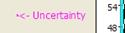
4.2.2.3 Uncertainty
area

According to the uncertainty
relation in the communication engineering and time-frequency analysis a precise
localization in time direction stands towards a simultaneously precise
localization in frequency direction. Both quantities can not be given
simultaneously exactly. So there is one uncertainty of the measurement in time
direction and one in frequency direction. The product of the two uncertainties
stretches the uncertainty area in the time-frequency domain. A decrease of the
area is desirable of course, it can be obtained by the built-in
DXP-transformation methods.
In order to gain a survey of the
uncertainty associated with the transformation settings quickly, TFA is
endowed with a face indication. On one hand it indicates the total area in
dependence of the scaling settings. And on the other hand it indicates the
uncertainty distribution that mainly turns out through the size of the time signal
interval coming in into the computation.
At the program start or after switching on this option the uncertainty area is
arranged for instance in the middle of the time-frequency domain and
magenta-coloured. It can be displaced, however, to every arbitrary point of the
program window with the mouse through the left mouse button. In Figure 4-2 the uncertainty area
![]()
is to be seen left of the
spectrum (above) respectively above the time representation (left hand). The
denomination „uncertainty" points at an uncertainty area with the form of
a point. This point appears very concentrated, because the spectrogram shows a
relatively big signal section both in frequency- and also in time direction.
A display-zoom with the
values:
- Time domain: 0.35
s to 1.0 s
- Frequency range: 50
Hz to 500 Hz
increases the detail level
and in this way also the „illustration" of the uncertainty area, as
following figure shows.
The uncertainty area is maybe
a little difficult to be found in the coloured environment of the
time-frequency domain.
Assistance: It lies a little
bit right above the XY Marker cross-hairs'.
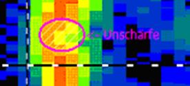
Figure 4‑5: Uncertainty area at transformation FFT, FFT-length: 1024
Caution: The physical
uncertainty area is not increased due to that zoom, only its representation.
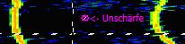
Increasing the FFT-length to
e.g. the value 4096 yields to the following spectrogram:
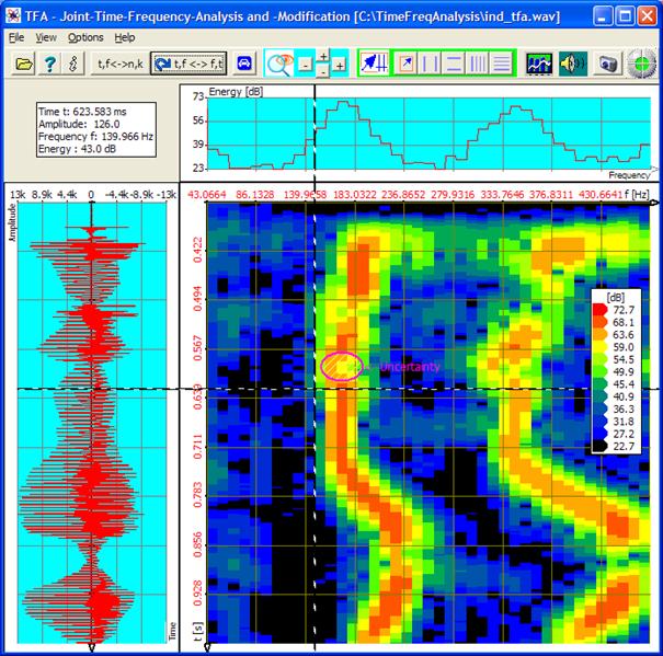
Figure 4‑6: Uncertainty area at transformation FFT, FFT-length: 4096
The uncertainty area
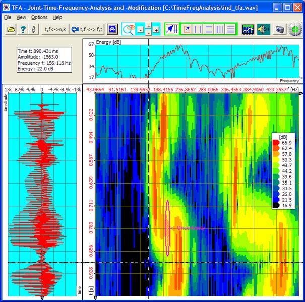
has grown around the factor 4
in direction of the time axis because a four times bigger time interval comes
into the calculation. In frequency direction on the other hand the size was
reduced around the factor 4.
The area itself is not
changed through enlargement or reduction of the FFT length, only the length
distribution. One can recognize, however, at least optically by means of the
two representations, that the indicated uncertainty area agrees in fact with
the uncertainty of the spectrogram.
What happens now with the
uncertainty area due to a selection of the transformation DXP-I?
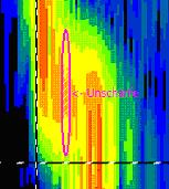
Figure 4‑7: Uncertainty area at DXP-I, resolution: 4096, time-window: 256 Samples
Also here the uncertainty
area is
![]()
is arranged a little
right-above the XY-Marker cross-hairs. One recognizes in agreement with the
spectrogram, that
- the small magenta-coloured circle-similar face is
just as extensive now in frequency direction, see Figure
4-6, because in both cases the FFT resolution is
4096,
- however the temporal extension is reduced around
the factor 8, what is associated with the reduction of the time window
interval of 4096 onto 256 samples.
Nevertheless please try it
out later yourselves as soon as the remaining control elements were also described
here!
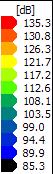
4.2.2.4 Level key
A spectrogram, therefore a
time-frequency analysis is a tridimensional representation. The third dimension
represents the energy which is colour coded. The level key, to be seen in the
right middle of the spectrogram in the figures above, is an assignment table
that relates colours corresponding to the energy steps.
Just like the representation
of the uncertainty area the level key legend can be moved to any place of the
program window with the mouse pointer by means of the left mouse button.
The setup of the level
colours is freely possible, see section 4.2.3.1 “Colours”.
4.2.2.5 Mouse
coordinates
If one moves the mouse
pointer over the signal presentations, an information sheet indicates the
signal quantities linked with the mouse coordinates. In case of the
time-frequency representation that are:
- Time
- Amplitude
- Frequency
- Energy
The mouse coordinate
information sheet can be moved with the mouse pointer by means of the left
mouse button anywhere in the area of the program window as well.
4.2.2.6 Progress
![]()
Depending on the performance
of the used computer some arithmetic operations may last a little longer. An
optical control for the process progress is a turning atom which appears at the
contact-place of the three signal presentations[2].
4.2.3
Options
TFA offers some options to an individual setup of the program:
- Colours
- Working directory
- Language/Sprache
- Settings
- Prog.-Start
with FFT
- DC-Offset-correction
- 1.0-Scaling
The settings are stored during the closing of the program.
4.2.3.1 Colours
![]()
With this command the
operation- and settings-window „Functions and parameters" is opened
directly with the tab "Settings":

Figure 4‑8: Operation window „Functions and parameters->Settings
“
In the upper half the colours of
- the level
legend
- many program
elements
can be configured.
4.2.3.1.1 Level-Colour-Assiociation
The first field „number of
level-colour-steps" is used for the setting of the colour resolution
of the energy in the time-frequency representation. The list „dB-levels"
contains as many dB-entries. Every level is separately eligible and may be
assigned a colour with the colour dialog (key ![]() ). With the key “Default” the level-colour-association
happens automatically in an intuitive color course:
). With the key “Default” the level-colour-association
happens automatically in an intuitive color course:
- High energy: Red
- …
- Low energy: Blue,
black
4.2.3.1.2 Colour
settings
The selection field „Colour
settings" lists all control elements that colour can be changed. Every
control element is separately eligible and may be assigned a colour with the
colour dialog (key ![]() ). With the key “Default” the colour assignment happens
automatically in the form of a colour proposal.
). With the key “Default” the colour assignment happens
automatically in the form of a colour proposal.
4.2.3.2 Working directory
![]()
There are functions in TFA
which write intermediate files onto the hard disk. With this option one can
pre-set the disk drive location.
4.2.3.3 /Language/
Sprache
![]()
TFA is written in the
national languages of German and English. With this option one chooses the
language.
4.2.3.4 Settings
![]()
With this command the
operation- and settings-window „Functions and parameters" is opened
directly with the tab "Settings", see Figure 4-8.
The settings contain graphic
and transformation properties defined by the user.
Several sets of settings can
be stored and loaded with the left two keys in the lower window half. With the
right key ![]() the factory settings can be reconstructed.
the factory settings can be reconstructed.
4.2.3.5 Prog.-Start
with FFT
During the termination of TFA
all settings are stored and loaded at a renewed start of program again. In the
case of the spectral transformation setting „DXP-I" that can be
disadvantageous because - maybe unintentional - after opening of a signal file
the slower DXP-transformation is immediately performed. This can be prohibited
through marking of this option.
4.2.3.6 DC-Offset-Correction
If this option is checked a
DC-offset will be removed while opening
a signal file.
4.2.3.7 1.0-Skalierung
If this option is checked
dependend on the file format the signals full scale is scaled to the value 1.0 while opening a signal file. So the
scale is not bounded to the file format.
Example: In case of a 16-Bit-PCM-Wav-file a sample with an amplitude of
32767 will be scaled to 1.0.
4.2.4
Help
TFA offers two possibilities for assistance:
- Documentation - This command indicates
this file.
- Info - Here you find the present program
version and reach
4.3
The short-keys
![]()
A basic principle during the
development of the TFA user interface is the use of the
screen area as efficient as possible. Therefore most control elements and input
fields are quartered in a separate window „Functions and parameters".
Saving place the short-keys offer access to the most important control elements
and if necessary open the window „Functions and parameters" for
advanced setting functions. Short-keys are available for following functions:
- Open
- Documentation
- Info
- Presentation
continuous / discrete
- Orientation
- Automatic scaling
- Area selection
- Vertical markers
- Horizontal markers
- Vertical Harmonic
marker
- Horizontal Harmonic marker
- Advanced XY-Marker functions
- „Zoom" -in and
-out
- Advanced Zoom / range functions
- Spectrum analysis settings
- Play / export
- DDC - Digital Down
Converter
- Graphic-export
- Status control
The functions are explained
in the following.
4.3.1
Open
![]()
This command opens a signal
file as described in section 4.2.1.1.
4.3.2
Documentation
![]()
The command indicates this document in the HTML-format.
4.3.3
Info
![]()
Here you find the present
program version and reach
4.3.4
Presentation continuous / discrete
![]()
In Digital Signal Processing
the number of a sample is associated with the its sampling time [s] by means of
the sampling frequency. Similar is valid for the number of a spectrum line and
the represented frequency [Hz]. With this command the presentation may be switched
between time [s] respectively frequency [Hz] and time sample number
respectively spectrum line number. One can e.g. purposefully find a wanted
sample or indicate values in its physical context.
4.3.5
Orientation
![]()
This command exchanges time
and frequency axis. Figure 4-7 would then turn as follows:

Figure
4‑9: Exchange of Orientation
4.3.6
Automatic Scaling
![]()
According to chosen signal
section the level distribution can be very different. On the one hand this
function adjusts the energy scaling of the time-frequency domain and the
spectral representation and on the other hand the amplitude scaling so, that
the diagrams are „well gained".
It is often worthwhile, to
call this function also e.g. after an alternation of
- the transformation method or its
parameters since due to the different uncertainty properties the existent
energy is distributed over a larger or smaller area or
- the signal selection.
The in the following
described control elements lie in the field
![]()
4.3.7 Area
selection
![]() .
.
For many TFA-functions it is
necessary to be able to select a certain signal range. The easiest possibility
for the selection of a signal range is maybe the drawing of a rectangle with
the mouse, similar like it is known from graphic arts software.
In order to activate this
function select mode, the area selection key is to be pressed. After that
selection rectangles can be stretched in all representations as following
example shows.

Figure 4‑10: Area selection in the time-frequency domain
Such an area one can then
e.g. enlarge (zoom), extract, export et cetera.
4.3.8
Vertical markers
![]()
Vertical markers are vertical
auxiliary lines in diagrams that can be positioned there with the mouse. After
pressing the key “Vertical markers” there are 2 markers (1’ and 2’) available
in every representation.
The marker positions appear
in a value table below the short-key-bar e.g. as follows:

Figure 4‑11: Value table for vertical markers
Apart from the marker
positions also the column (2’ -1’) is to be seen. It shows the distance of the
two markers.
The marker position
may be adjusted with the mouse or placed exactly via entry of a wanted
numerical value into the white fields.
Notice: The activation of
the vertical markers deactivates other vertical markers and the area selection,
see below.
4.3.9
Horizontal markers
![]()
Horizontal markers are
horizontal auxiliary lines in diagrams that can be positioned there with the
mouse. After pressing the key „Horizontal markers” there are 2 markers (1’ and
2’) available in every representation.
The marker positions appear
in a value table below the short-key-bar comparable to Figure 4‑11: "Value
table for vertical markers”, see above.
Also here is valid:
Apart from the marker
positions also the column (2’ -1’) is to be seen. It shows the distance of the
two markers.
The marker position
may be adjusted with the mouse or placed exactly via entry of a wanted
numerical value into the white fields.
Notice: The activation of
the horizontal markers deactivates other horizontal markers and the area
selection, see below.
4.3.10
Vertikal harmonic marker
![]()
A Harmonic-marker consists of
a band of markers that are characterized by two quantities:
- Marker start - the position of the
first marker of a band
- Distance – Distance of two neighbouring
markers
Harmonic markers are used in
order to be able to measure cyclical processes over several cycles.
An example is the measurement
of a digital data stream in the case of which the bit length is constant.

Figure 4‑12: Measurement exampe with „Vertical harmonic markers“
The marker positions appear
in a value table below the short-key-bar comparably Figure 4‑11: „Value table for vertical markers", see above.
One reads off that the
temporal bit-distance of the frequency shift keying is 4,16 ms, which
corresponds to a modulation rate of about 240 Bd. By the way: The example shows
a FSK radio transmission method, where the information transmission reclines in
the keying of two frequencies.
Notice: The activation of
the vertical harmonic marker deactivates other vertical markers and the area
selection, see below. However, the vertical harmonic marker may be combined
with horizontal markers.
4.3.11 Horizontal
harmonic marker
![]()
The former section explains
the vertical harmonic marker. Corresponding is valid for the horizontal
harmonic marker.
Notice: The activation of
the horizontal harmonic marker deactivates other horizontal marker and the area
selection, see below. However, the horizontal harmonic marker may be combined
with vertical markers.
4.3.12
Advanced XY-Marker functions
![]()
The value table of the marker
positions indicated in the main window is maybe printed in a little small way
and according to the adjusted size of the graphics through insertion of
so-called scroll bars unclear.
With this command or via a
right click with the mouse above a graphic the operation- and settings-window
„Functions and parameters" is opened directly with the tab
"XY-Marker":

Figure 4‑13: Operation window „Functions and parameters->XY-Marker“
Here the marker positions may
be read off conveniently and postponed through input of other values.
The keys above the value
table correspond to the keys in the short-key-bar of the main window, cf.
sections 4.3.7 “Area selection" to 4.3.11 „Horizontal harmonic marker“.
The in the following
described control elements lie in the field
![]()
4.3.13 „Zoom“-in and -out
![]()
All three representations can
be zoomed in or out in both their axial directions:
- Time
representation: Time and
amplitude
- Spectrum: Frequency and
energy
- Time-frequency: Time and frequency
A zoom-in (key ![]() ) presupposes,
that the new boundaries of the indicated section are defined via markers or the
area selection see, above. With a zoom-out (key
) presupposes,
that the new boundaries of the indicated section are defined via markers or the
area selection see, above. With a zoom-out (key ![]() ) the indicated
interval doubles, increasing at both boundaries evenly.
) the indicated
interval doubles, increasing at both boundaries evenly.
There are four zoom-keys
which are horizontally respectively vertically arranged. With these it can be
zoomed in both directions independently by each other.
4.3.14 Advanced zoom/boundary
functions
![]()
With this command the
operation- and settings-window „Functions and parameters" is opened
directly with the tab „Zoom / Range“:

Figure 4‑14: Operation window „Functions and parameters->Zoom / Range“
In the left field there are
to see the four zoom-keys again explained in the former section ![]() and
and ![]() .
.
In addition the window
contains also the keys ![]() and
and ![]() that are arranged diagonally. These represent
a combination of horizontal and vertical zoom.
that are arranged diagonally. These represent
a combination of horizontal and vertical zoom.
In the right field the
current scalings of the indicated intervals of amplitude, time, frequency and
energy are written. These fields are editable, so that a zoom can be carried
out directly and precisely there.
With the help of the keys ![]() the borders of the viewed time interval can be
scrolled in the future and the past.
the borders of the viewed time interval can be
scrolled in the future and the past.
The key ![]() calls the function 4.3.6 „Automatic Scaling“.
calls the function 4.3.6 „Automatic Scaling“.
Tip: If „DXP-I"
and „DXP-II" is chosen as spectral transformation method the picture
buildup can last longer. Before the performing of multiple zooms it is
recommended to change temporary to transformation method „FFT" in order to
return at the end to „DXP".
4.3.15
Spectrum analysis settings
![]()
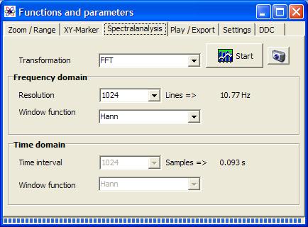
With this command the
operation- and settings-window „Functions and parameters" is opened
directly with the tab „Spektralanalysis“:

Figure 4‑15: Operation window „Functions and parameters ->Spektralanalysis“
The spectrum analysis settings and control elements include:
- Transformation
- Start
- Graphic-export
- Frequency
domain with resolution and window function
- Time domain
with time window and window function
These shall be explained in the following.
4.3.15.1
Transformation
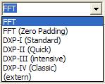
Four transformation methods are available:
- FFT
- FFT with zero padding
- DXP-I (Standard)
- DXP-II (Quick)
- DXP-III (intensive)
„FFT" is the usual Fast
Fourier Transform where a time interval of n samples (in the real valued case)
leads to n/2 spectrum lines.
The transformation „FFT
(Zero padding)" is a FFT at which for n/2 spectrum lines not n samples
but base-2 power fractions of n samples go into the transformation. The samples
being lacked by the FFT then are replaced by null values. A Zero-Padding-FFT
offers for a certain sample number a compared to the FFT finer scanning of the
frequency spectrum. However, there is no improvement of the resolution or
decrease of the uncertainty.
Unlike the Zero-Padding-FFT „DXP-I“, „DXP-II“, „DXP-III“ und „DXP-IV“ are signal expanders that do not replace the missing samples with zeros,
but with in fact calculated values. The different versions bring out
a different trade-off between calculation time and accuracy:
- DXP-I is a good
choice for general analysis (Standard).
- DXP-II calculates
faster, but less precise. At signal frequencyies near DC (f = 0 Hz)
- DXP-II may
calculate even more precise than DXP-I.
- DXP-III is a bit
more accurate but affords double calculation time.
- DXP-IV is an older
version kept for comaparision purpose.
Notice: The transformation method „(extern)" is not implemented in
version V2.x yet.
4.3.15.2
Start
![]()
This key starts the
calculation of the time-frequency representation. According to chosen
transformation method and size of the display window this can last longer. The
progress bar at the lower window border informs of the degree of the finishing.
4.3.15.3
Graphic-Export
![]()
For documentation purposes a
graphic-export into other Windows application is possible as usually by
pressing the key combination <ALT-Print>.
Additionally a file export is
available to export the time-frequency representation as a bitmap graphics file
(format „BMP”). This command opens a „File-Save-As…"-Dialog to name and
save the graphics file.
The command is identical with
the one described in section 4.3.18. At this place the key only increases the operating
convenience.
4.3.15.4
Frequency domain
This dialog field offers
settings that primarily affect the frequency domain:
- Resolution
- Window function
4.3.15.4.1
Resolution
The resolution whose value is
adjustable in a selection box indicates the number of lines of a spectrum,
therefore the node number of the spectrum. According to the sampling rate the
frequency distance [Hz] of two neighbouring lines is joined with the line
number. This value is to be seen to the right next to the selection box.
4.3.15.4.2
Window function
In the field of general spectrum
analysis window functions are in common use. They weight a time interval of
„resolution”-many samples. Such a window function can have in principle following
figure:

Figure 4‑16: A possible window funkction for weighting a time interval
Many different types of
window functions exist. In TFA some especially frequently used ones are
implemented:
- „Rectangle"
- „Hamming"
- „Hann"
- „Blackman"
- „Bartlett"
These and their spectrum
analysis properties are extensively described in the literature and shall not
be explained here in detail therefore.
4.3.15.5
Time domain
This dialog field offers
settings that apply indeed in the time domain, however, have also effect on the
spectral representation. The are:
- Time interval
- Window function
4.3.15.5.1
Time interval
The time window, that is the number
of samples of the time interval coming in into the transformation, is
adjustable with a further selection box. In case of transformation methods like
„FFT" this selection is not possible because the time interval is given by
the resolution already. Other transformation methods like
„FFT-(Zero-Padding)" or the „DXP"- transformation methods allow the
separate choice of the time interval.
According to sampling rate a
certain time interval [s] is associated with the time window size. This is to
be seen to the right next to the selection box.
4.3.15.5.2
Window function
As in the case of the
category „Frequency domain" there are are the same function types, see
above:
- „Rectangle"
- „Hamming"
- „Hann"
- „Blackman"
- „Bartlett"
4.3.15.6
Further explanation of the settings
In TFA time-frequency analyses are possible,
that are not known in the case of other products and therefore are not
familiar. This section explains the analysis principle in case of the DXP-transformation
methods.
Supposed:
- A signal Z exists in time domain, at which Z is
defined through the choice according to section 4.3.15.5.1 “Time interval„.
- This time interval is windowed according to
section 4.3.15.5.2 “Frequency
domain„ e.g. with a window function of the type
„Hann".
Then in the following figure
the upper curve shows just this windowed time signal.
The time signal is expanded
by the means of the DXP-transformations onto N values, these are to be seen in
following figure in the lower curve.
Figure 4‑17: Expansion
of a time interval Z (above) onto N samples (below
Figure below: The onto
N-values (N = resolution according to section 4.3.15.4.1 “Resolution“) expanded time signal (red) is windowed according to
section 4.3.15.4.2 “Window
function" (green). The windowed time signal (blue) is
transformed with the N-Points-FFT.
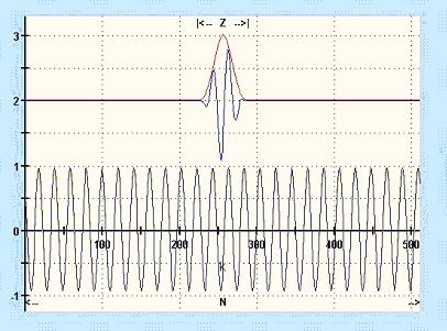
Figure 4‑18: Windowing of the expanded time interval at N Samples
In this manner one gets a N
node spectrum that arises from a Z-samples time interval at which Z<<N
is. In that a special feature of TFA lies.
4.3.16 Play
/ Export
![]()
With this command the
operation- and settings-window „Functions and parameters" is opened directly
with the tab „Play / Export“:

Figure 4‑19: Operation window „Functions and parameters ->Play / Export“
This command category is used
to select signal intervals by means of the area selection or the XY-markers
(see sections 4.3.7 to 4.3.9) directly in the representations
- Time domain - Selection of a time
interval at full frequency bandwidth
- Frequency domain - Selection of a
frequency range with complete original time interval
- Time-frequency domain - Selection
of a time interval and simultaneously frequency range
and to extract it time-
and/or frequency band-restricted and then
- to indicate it in a new TFA instance or
- to export it as a WAV- or TFA signal file.
During this process further
signal modifications are possible if applicable.
The „Play / Export”-settings and control element include:
- Playback functions
- Envelope, magnitude
- Lower level
threshold
- Speed vs. Quality
- TFA-instance
- Export
- Cancel
These shall be explained in
the following. As said they presuppose a preceding area selection in one of the
graphics.
4.3.16.1
Playback functions
![]()
This keypad is used to play back
the selected signal range via the loudspeakers of the PC system like it is
usual in many windows applications. There are the commands
- Start
- Pause
- Stop
- Back
implemented. According to
selected graphics representation the computation of the signal to be played can
last longer. The simple selection in the time domain is natural quickly
possibly while selections in the time-frequency domain can last longer
according to the size of the time interval. The progress bar at the lower
window border informs of the degree of the finishing.
4.3.16.2
Envelope, magnitude
![]()
If this box is checked, TFA will calculate the signals
envelope. This is used e.g. for further analysis of modulation spectra with a
new TFA instance or other analysis tools.
4.3.16.3
TFA-instance
![]()
Instead of playing the
selected signal via the loudspeakers of the PC system, one can start a new TFA-instance with this key. That means,
a new TFA program window is opened that shows already the selected signal.
As many TFA-instances as desired can be started in parallel. Only the
system resources state a limitation here of course.
4.3.16.4
Export
![]()
This command operates as the
two mentioned before. The output of the selected signal is carried out as WAV-
and TFA-file via a "file-save-as… "-dialog. In case of WAV there are
several subformats, e.g. 16-Bit-PCM, 24-Bit-PCM, 32-Bit-PCM and 32-Bit-FLOAT.
4.3.16.5
Cancel
![]()
As already
mentioned the computation of the signal extraction can last longer. With this
key the process can be stopped.
4.3.16.6
Lower level threshold
In case of a selection in the
representations
- time-frequency
domain
- frequency domain
the specification of an
absolute lower level threshold is possible. For this it is to mark the check
box and to enter a wanted level threshold in the [dB]-field.
Lines with energy values
below this threshold are set on the value Zero – like it is done in any case
with lines outside of the selection area.
That means especially for the
filtering in the time-frequency domain, that also weaker signal parts within
the bandpass filter area (!) being able to be eliminated. This
behavior appears as a frequency-agile bandpass filter that adjusts itself to
the signal contents - a further special feature of the software TFA!
Also in case of the filter
selection in the frequency domain representation this function can be useful,
however, the probability for the case that all line energies are below the
threshold during the entire original signal is usually considerably smaller
than if the time dependence is considered additionally.
4.3.16.7
Speed vs. Quality
In the case of a selection in
the representations
- time-frequency
domain
- frequency domain
the adjustment of a
compromise between processing speed and the achieved result quality is
possible.
Check box „Use always Fast
Fourier over the complete signal":
The highest speed is achieved
by:
- Deactivation of a possibly chosen
DXP-transformation for the benefit of the FFT-transformation
- Computation over the complete signal without
considering the temporal behaviour. Notice: Then a possible chosen low
level suppression can not operate time-agilely anymore. Instead of this
the consideration of the average signal level occurs.
For this the check box is to
be marked.
Slow / fast - control
If the above mentioned check box is not marked, also in case
of DXP-transformation the speed can be increased through a single
transformation supplying several samples. Through that the time reference of
the transformation suffers a little which, however, mostly does not disturb
because it is a question of only some ten samples.
The number of the samples
used with every single transformation can be varied with the slider and thus
the speed can be adjusted between „Slow" and „Fast".
4.3.17 DDC
– Digital Down Converter
![]()
From version V2.x TFA
is equipped with a Digital-Down-Converter (DDC).
What is the primary benefit
of a DDC?
The great advantage of a DDC
is the possibility of sampling rate reduction. In the case of a given spectral
resolution reduced signals can be surveyed more precisely in frequency
direction because with the decimation of the sampling frequency the mode
separation of two spectrum lines sinks. That is in particular favourable in
case of the DXP-transformations because their adjustable frequency resolution
is restricted on 4096 lines.
Example:
Situation: A signal sample
of a physical phenomenon includes interesting signal components in the
frequency range 250 kHz +/- 5 kHz. The high center frequency forces to a high
sampling rate of e.g. 1 MS/s.
Consequence: Then the mode
separation of two spectrum lines is about 244 Hz at a frequency resolution of
4096. So the to be examined 10 kHz frequency band is presented only through
about 40 lines.
Relief:
Digital-Down-Conversion of the signal with shifting down the frequency band
around 245 kHz and reduction of the sampling rate from 1 MS/s to e.g. 40 kS/s. In
this way the frequency resolution is about 10 Hz or rather about 1000 lines.
Therefore the DDC belongs to
the indispensable equipment of a spectrum analysis system.
To support a clear
arrangement of the main window, no own access point is available there for the
DDC. The DDC can be obtained via the operation-
and settings window „Functions and parameters” and the tab „DDC":

Figure 4‑20: Operation window „Functions and parameters ->DDC“
This command category is used
to select signal intervals by means of the area selection or the XY-markers
(see sections 4.3.7 to 4.3.9) directly in the representations
- Time domain - Selection of a time
interval at full frequency bandwidth
- Frequency domain - Selection of a
frequency range with complete original time interval
- Time-frequency domain - Selection
of a time interval and simultaneously frequency range
and to extract it time-
and/or frequency band-restricted and then
- to indicate it in a new TFA instance or
- to export it as a WAV- or TFA signal file.
In addition to the extraction
as an ordinary time signal the calculation of the instantenous values is
possible for eq. modulation spectra analysis.
The group of „DDC”-functions
is related to the group „Play / export", however, there are fundamental
differences. The group of „DDC”-functions is used for following operations:
- Selection of a signal range with band-pass
filtering
- Frequency shift e.g. to shift of
inaudible high-frequency contents into the acoustic range
- Reduction of the sampling rate for the
decrease of the quantity of data and to rise of the spectral gauging
accuracy
- Transformation of a real-valued signal into an
analytical complex-valued one as an alternative e.g. to the
Hilbert-transformation. In the complex case many methods of measurement
exist which are denied to real-valued signals.
- Transformation of a complex-valued signal into a
real-valued one
- Calculation of instantenous values
The „DDC”-settings and controls include:
- One /two channel file
- Mixer
frequency
- Decimation factor
- Automatic
DDC-setting
- Instantenous
values
- TFA-instance
- Export
These shall be explained in
the following. They presuppose as said a preceding area selection in one of the
graphics.
4.3.17.1
One-/Zwo channels
![]()
Here it is to be specified
whether the DDC result shall be real-valued or complex-valued. Complex-valued
files require the setting „2".
4.3.17.2
Mixer frequency
![]()
This is the negative or
positive frequency shift a selected signal will be transposed. Depending on,
whether frequency specifications are „continuous" or „discretely" (selected
according to section 4.3.4 or the key ![]() ), one enters the
frequency shift in [Hz] or in frequency lines of the spectrum.
), one enters the
frequency shift in [Hz] or in frequency lines of the spectrum.
4.3.17.3
Decimation factor
![]()
With the selection of a
frequency range a band limitation is associated. With a frequency shift towards
f=0 the signal bandwidth respectively the highest occurring signal
frequency is reduced again. According to the sampling theorem[3] the sampling frequency has to be only at
least twice of the highest signal frequency. One can reduce the sampling
frequency where appropriate. A decimation factor (> 1) may be
specified in this field.
4.3.17.4
Automatic
setting of the DDC
![]()
In dependence of the desired
number of channels there is a usual case for which TFA can carry out the
DDC- setting itself or suggest it.
- Real-valued
1- channel result file: This case describes the desire, that a
selected higher frequency band is mixed down so that the lowest
frequency appears in the frequency zero position. The sampling rate
can be reduced then concerning the new highest signal frequency.
Example: Making audible of
a signal outside the acoustic range.
- Complex-valued
2- channel result file: Here the middle of the selected
higher frequency range is supposed to appear in the frequency zero
position.
Example: Digital modulated
communication engineering signals (ASK, PSK, FSK) which can be analyzed in
complex base band situation better. The sampling rate reduction can refer to
the modulation rate
Pressing the key fills the two DDC input fields.
4.3.17.5
Instantenous values
![]()
Eg. for the analysis of
modulation spectra instantenous values are used instead of the time signal.
Dependend on the modulation type one of the 3 options is to be marked.
4.3.17.6
TFA-instance
![]()
With this key the DDC result
can be indicated in a new TFA-instance.
That means, a new TFA program window is opened that shows
already the selected signal.
As many TFA-instances as desired can be started in parallel. Only the
system resources state a limitation here of course.
4.3.17.7
Export
![]()
This command operates as the
one mentioned before. The output of the selected signal is carried out as WAV-
and TFA-file written to disk via a "file-save-as… "-dialog. In case
of WAV there are several subformats, e.g. 16-Bit-PCM, 24-Bit-PCM, 32-Bit-PCM and
32-Bit-FLOAT.
4.3.18 Graphic
export
![]()
For documentation purposes a
graphic-export into other Windows application is possible as usually by pressing
the key combination <ALT-Print>.
Additionally a file export is
available to export the time-frequency representation as a bitmap graphics file
(format „BMP”). This command opens a „File-Save-As…"-Dialog to name and
save the graphics file.
The command is identical with
the one described in section 4.3.15.3. At this place the key shall only increase the
operating convenience.
4.3.19
Status control
![]()
If the indication shines
green, TFA is in idle status. If it shines red, computations are not
finished yet. If the operation window
„Functions and parameters” is opened the progress bar at the lower window
border informs about the degree of the finishing.
5
Practices
TFA and DXP are new, still little spread tools, that are not - that
is preceded - difficult to master. However, a little bit of practice and also
knowledge and experience is useful in order to be able to draw the full benefit
from that. Who is not yet so familiar to DXP, this short chapter is warmly
recommended to. It offers an entrance, and is considered as a starting point
for the exploration of the own signal material.
The solving of the given tasks is nonessential. More important is the
practice with the functions of TFA.
Representative for the almost infinite application field of time
frequency analysis some topics will be handled which maybe especially often
occur in theory and practice in a comparable sense and therefore were already object
and example of this documentation. They are:
Time frequency analysis
·
Speech signal: F0-analysis in natural language
·
Communication engineering: FSK-signal with shift- and
modulation rate measurement
Filtering
·
Speech signal: Extraction of the F0-oscillation
·
Communication engineering: Extraction of a FSK-signal
Frequency translation
·
Speech signal: Making audible a discant voice
component
·
Communication engineering: Conversion of a real-valued
signal into the complex base band
5.1
Time frequency analysis
Purpose of this section is to
show, how a first small knowledge about the signal composition changes from
step to step successive to a clean overall picture. Very important is to
bring up the measurement close to the border of Technical Uncertainty
Relation cautiously because TFA can not unfold its strengths before then.
And not till then a analysis precision will occur that is not accessible with
conventional procedures.
A basic principle is derived
from that:
TFA is suitable for
every kind of the spectrum analysis and time frequency analysis. However, the
abilities of DXP do not become visible before the signal analysis
situation requires this precision. Indeed this is mostly the case at time
frequency scenarios, however, if these lie far from the uncertainty relation, DXP
is not necessary and the in TFA also implemented FFT equivalent. In the
extreme case of the analysis of a sine continuous tone DXP does not
cause any advantage compared to a FFT-analysis.
Tip 1:
To be able to graphically recognize
a sharpness-/uncertainty effect at all, it is important that in TFA a
time signal area became zoomed, that is so small, that the uncertainty area,
cf. section 4.2.2.3 “Uncertainty
area”, is clearly to see. Otherwise the uncertainty possibly
may not be evaluated due to the restricted resolution of the PC monitor and the
eye.
Tip 2:
At first the most important
DXP-setting is the choice of the correct time interval according to section 4.3.15.5.1 “Time interval". If possible the time window size should be as
large as a signal interval may be considered as stationary. Examples: A
stationary signal interval can have for instance the length of a speech sound
or e.g. half the bit length of a communication signal.
The FFT analysis is suited
well as a Pre-analysis, in order to find out a first value for the DXP
time interval and, whether there is a time-frequency analysis problem actually
at all. For this one can test several FFT-lengths. If it turns out that at
smaller FFT lengths a time-frequency dependant energy distribution appears,
then this would be a first choice for the DXP time interval after a change to
the DXP-I-transformation or DXP-II transformation method.
Tip 3:
After switching on the
DXP-transformations
- one takes the just appraised time interval as a
fist basis (furthermore a Hann-window is mostly a good choice),
- adjusts the frequency resolution to the same (if
the frequency resolution is identical the time interval, then DXP works as
FFT) and
- increases the frequency resolution successively according
to section 4.3.15.4.1 “Resolution„.
Then the frequency contents
should appear exactly as well.
Tip 4:
Based on the fact of this
constellation one can experiment with different time interval sizes, window
functions and resolutions. Thereby one pays attention to the uncertainty area
which must match to the signal temporally and which then indicates the
frequency-uncertainty spectrally.
With these 4 tips a
TFA-DXP-time frequency analysis succeeds.
5.1.1 Speech signal: F0-analysis in
natural language
Question: Which is the
fundamental frequency of the voice from file „ind_tfa.wav"
at the time t =
0,77 s?
Answer: At this time the
fundamental frequency F0 is f = 188,4 Hz.
In order to obtain an answer, one can run through e.g. following steps:
1. Step – Opening the file and representing it clearly
One
- opens the
file „ind_tfa.wav”

- marks all
view-options
- sets in the
window „Functions and parameters->Spektralanalysis” (
 ) the
transformation method to „FFT"
with a resolution 1024
) the
transformation method to „FFT"
with a resolution 1024 - presses the key „Start"
- presses the
key „automatic scaling"
 at the main window
 - presses possibly
the keys „Presentation continuously / discrete"
 and/or „Orientation"
It will appear the following
or a very similar program window. According to PC system the figure can differ
a bit and of course e.g. the XY-marker depends on the position of the mouse
pointer, and so forth.
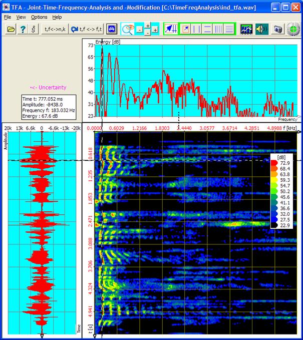
Figure 5‑1: File „ind_tfa.wav“, FFT-analysis, resolution 1024 Points
The XY-marker is positioned
already approximately at the place of interest. One reads in the area „mouse
coordinates”, cf. section 4.2.2.5 “Mouse coordinates":
t = 777,052 ms f = 183,032 Hz
That is not very exactly yet,
because already the restricted graphics resolution of the monitor is noticeable
here. A „zoom-in" according to section 4.3.13 „Zoom“ will help. That happens in the next step.
2. Step - Zoom into the time-frequency domain’s area of interest
For that there are several possibilities:
- Direct
setting of the indicated area via the key
 , cf. section
4.3.14 “Advanced zoom/boundary function"
, cf. section
4.3.14 “Advanced zoom/boundary function" - area
selection
 according to section 4.3.7 and zoom
 - use of the
„Vertical markers"
 and „Horizontal markers"
 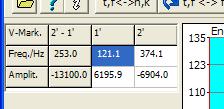 according to sections 4.3.8 and 4.3.9
The last method is maybe a
little complicated, but in this case one learns the dealing with the markers,
for which up to now this documentation still gave no deeper going explanation.
The markers are conveniently
to move with the mouse. Here they shall be positioned, however, via keyboard
inputs so that the following representations here and in this practice look
homogeneous.
For
the zoom
- one presses the keys and for the activation of the vertical and
horizontal markers,
- one enters 0,5 s to 1,0 s as the time interval
into the marker value table,
- one enters 0 Hz to 600 Hz as the frequency range
into the marker value table.
That can happen directly in
the program main window. Then the marker value table looks as follows, whereby
only the two middle rows are of interest:
After that the program window
is shown similarly as in the following figure:
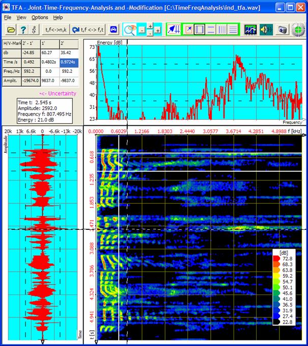
Figure 5‑2: Positioning of horizontal and vertical markers
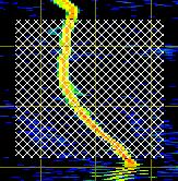
After a zoom-in the area enclosed
between the markers ...
... expands over the entire
time-frequency domain.
The zoom can be done with the
two ![]() -keys according to
section 4.3.13 or “Advanced zoom/boundary function„ (
-keys according to
section 4.3.13 or “Advanced zoom/boundary function„ (![]() ) according to
section 4.3.14. In case of the first possibility one presses
) according to
section 4.3.14. In case of the first possibility one presses
- the two of them
 -keys in the
main program window, to arrange a vertical and a horizontal zoom into the
marked area. Notice: Possible you must click with the left mouse button
somewhere into the time-frequency domain for TFA recognizes this
representation to be adapted. The latter happens automatically during the
positioning of the markers by mouse pointers.
-keys in the
main program window, to arrange a vertical and a horizontal zoom into the
marked area. Notice: Possible you must click with the left mouse button
somewhere into the time-frequency domain for TFA recognizes this
representation to be adapted. The latter happens automatically during the
positioning of the markers by mouse pointers. - the keys and for the deactivation of the vertical and
horizontal markers
- the key
„automatic scaling" , to adapt
the scaling onto the new representing-area.
The result of the zoom is:
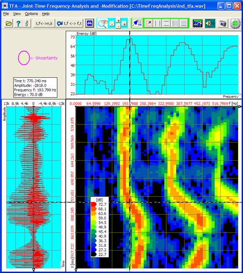
Figure 5‑3: Zoom in the time-frequency domain
One
pays attention to
- the uncertainty area
 , which
expresses the reliability of the spectrogram after the zoom
, which
expresses the reliability of the spectrogram after the zoom - that now a F0- value of f = 193,799 Hz is just as
plausible as the before taken value of f = 183,032 Hz. The reason lies in
the FFT owning a line mode separation of 10,77 Hz during the resolution of
1024 points.
3. Step - Attempt: Rise of
the measurement accuracy in time- and frequency direction
In general the measurement
accuracy of the FFT may be risen through an increase of the FFT length,
therefore an increase of the resolution. What happens if the FFT-resolution is
increased from 1024 to the value 4096 shows following figure.
For
this
- one sets in
the window „Functions and parameters->Spektralanalysis” () the
transformation method „FFT" with a resolution of now 4096
- one presses
the key „Start"
- one presses
the key „Automatic scaling” in the main window after finishing of the
spectrogram
The result of the higher
FFT-resolution shows the figure after next. The accuracy became worse in both
coordinate directions. The reason is that with the rise of the FFT-resolution
the uncertainty area was changed in
![]() respectively with spectrogram set aside
respectively with spectrogram set aside 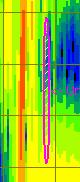
Figure 5‑4: Uncertainty area at a 4096-Points-FFT
In frequency direction the
uncertainty area became around the factor 4 more narrowly indeed, but in time
direction four times so long. At places in the time-frequency domain where the
signal frequency changes and therefore no stationarity is given anymore this
FFT analysis can neither express the frequency- nor the behaviour in time.
One can find, that the rise
of the FFT resolution from 1024 up to 4096 points lets become the analysis more
inaccurately:
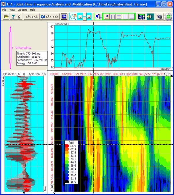
Figure 5‑5: FFT-analysis, resolution 4096 points
It is clear that therefore
also the opposite which is the decrease of the FFT-resolution from 1024 to e.g.
512 points can not increase the analysis accuracy. One even tries that out by
oneself!
Now it is time to turn on the
DXP transformation method.
4. Step - Rise of the
measurement accuracy in time- and frequency direction with DXP
In the former sections it was
to be recognized that an analysis time interval of 1024 samples is at least to
be preferred to a value by 4096.
- Therefore an analysis time interval of 1024
values shall serve as a start value for the DXP-analysis.
- Since DXP is only reasonable if the frequency
range resolution is bigger than the value of the analysis time interval, a
resolution is immediately applied by 4096.
In order to carry out the
transformation correspondingly the following is to do:
One
- sets the
transformation method in the window „Functions and parameter->Spektralanalysis”
() to
„DXP-I" with a frequency resolution of 4096 lines and “Hann” as the
windowing function,
- selects in
the field “Time domain” the time interval to the value 1024 Samples and
again a “Hann”-window,
- presses the key „Start" and
- presses the
key „Automatic scaling” in the main window after finishing of the
spectrogram.
The result of the
DXP-transformation is to be seen in the next figure. One pays attention to
- the change of the uncertainty area from
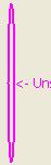 to
to  , what is
achieved through the reduction of the analysis time interval,
, what is
achieved through the reduction of the analysis time interval, - that the spectrogram does still not comply
to the vision according to known basics of the voice generation.
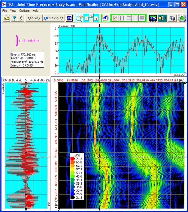
Figure 5‑6: DXP-I-analysis, resolution 4096 points, time interval 1024 samples
Now, what’s responsible for
impression that the spectrogram does still not seem to be clean?
The reason is simple: The
adjusted analysis time window (1024 samples) is still too big, because the
pitch change in this time span is enormous. The calculated spectrum lines
represent all frequency pitches that appeared.
As said at DXP the
specification of the analysis time interval is independent of the specification
of the frequency resolution. Therefore one can simply reduce analysis time
interval.
For this the following is to
be done:
- In the window
„Functions and parameter->Spektralanalysis” () – field
“Time domain” one sets the time interval to a value of 256 samples, the
“Hann” window remains.
- One presses
the key „Start" .
- Again, one
presses the key „Automatic scaling” in the main window after finishing of the
spectrogram.
The result of the
DXP-transformation is to be seen in the next figure.
Figure 5‑7: DXP-I-analysis, resolution 4096 points, time interval 256 samples
One pays attention to
- the change of the uncertainty area from to
 , what is
achieved through the repeated reduction of the analysis time interval,
, what is
achieved through the repeated reduction of the analysis time interval, - that now a F0-value f = 188,416 Hz is to be read
quite simply and exactly.
Even more simply and more
precisely the F0-measurement succeeds after a further temporal zoom. As further
above described, in the following a zoom is carried out into the time interval
of 0,7 to 0,84 s:
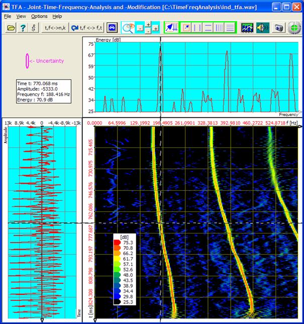
Figure 5‑8: DXP-I-analysis, resolution 4096 points, time interval 256 samples,
Zoom
Along the way: The transformation DXP-II
supplies similar results of analysis as DXP-I. The quality is not quite as
well, for that DXP-II works considerably more quickly. Following figure shows
DXP-II under the same conditions as above.
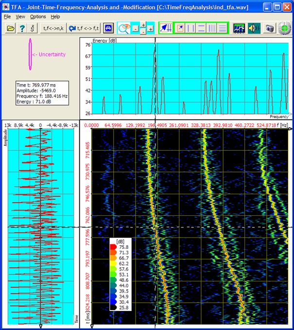
Figure 5‑9: DXP-II-analysis, resolution 4096 points, time interval 256 samples,
Zoom
5.1.2
Communication
engineering: FSK-signal with shift- and modulation rate measurement
Question: Which are
the frequency shift and the modulation rate in the FSK-signal
given in file
„ind_tfa_2.wav"?
Answer: The shift is ∆f =
170,9 Hz.
The modulation
rate MR = 231,48 bd.
Notice:
This signal file is complex-valued material. That means, in the format of a
stereo Wav file a two channel signal is contained, at which the two channels
are used for real part and imaginary part. Characteristic for complex-valued
signals is that the frequency axis shows also negative frequency. The frequency
range of a complex-valued signal ranges from –samplingrate/2 to
+samplingrate/2. In case of real-valued signals the frequency range is 0 Hz to
+samplingrate/2.
In order to achieve the answer, one can carry out e.g. following steps:
1. Step – Opening file and representing it clearly
One
- opens the
file „ind_tfa_2.wav” ,
- marks all
view-options,
- selects the
transformation method „FFT" in the window „Functions and
parameters->Spektralanalysis” () with a
resolution of 1024,
- presses the key „Start" ,
- presses the
key „Automatic scaling” in the main window,
- presses
possibly the keys „presentation continuously / discrete" and/or „Orientation" .
The following or a very
similar program window will appear. According to PC system the figure can differ
a little, and of course e.g. the XY marker depends on the position of the mouse
pointer, and so forth.
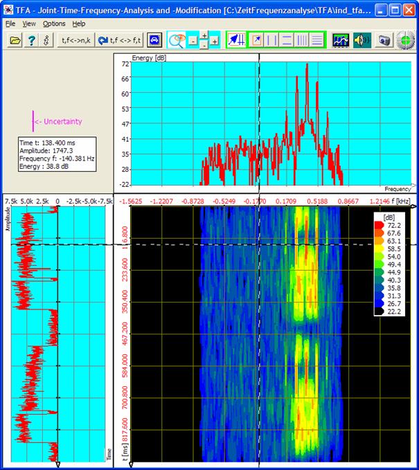
Figure 5‑10: File „ind_tfa_2.wav“, FFT-analysis, resolution 1024 points
The signal section obviously contains
4 signal blocks, of which each two adjoin closely. It is presumed that the
composition of the two double blocks is qualitatively identical. For the
further analysis one can arbitrarily decide e.g. for the upper one.
That happens in the next
step.
2. Step – Zoom into time frequency intervals
In order to select the upper
double block, there are again several possibilities:
- Direct
specification of the indicated area via the key , cf. section
4.3.14 “Advanced zoom/boundary function"
- Area
selection according to section 4.3.7 with drawing of a selection rectangle in the
time domain or in the time-frequency domain and after that zoom
- Use of the
„Vertikal markers" and „Horizontal markers" according to sections 4.3.8 and 4.3.9
Again the last method is
selected with the positioning of the markers by keyboard entries so that the
following representations here and in the exercise look homogeneous.
The following is to be done
to zoom:
One
- presses the keys and for the activation of the vertical and
horizontal markers,
- enters 0 s to 0,44 s into the marker value table
as a time interval,
- enters 0 Hz to 700 Hz into the marker value table
as a frequency range,
- presses the two -keys in the
main program window, to arrange a vertical zoom and a horizontal zoom into
the marked area (Notice: Possible you must first click anywhere into the
time-frequency domain with the left mouse button for TFA does
recognize the graphic to be adapted. The latter happens automatically
during the positioning of the markers by mouse pointers),
- presses once again the keys and for the deactivation of the vertical and
horizontal marker and
- the key
„Automatic scaling" , to adapt
the scaling onto the new representing- area.
The result of the zoom is to
be seen in the next figure. The uncertainty area  shows that the chosen analysis time window is
much too large in respect of the present signal, because at least the pause
between the signal blocks is much shorter. Therefore the pause is indeed to be
recognized in the time domain but not in the time-frequency domain.
shows that the chosen analysis time window is
much too large in respect of the present signal, because at least the pause
between the signal blocks is much shorter. Therefore the pause is indeed to be
recognized in the time domain but not in the time-frequency domain.
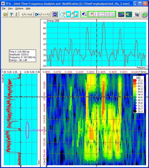
Figure 5‑11: Representation after zoom, FFT-analysis, resolution 1024 points
Nevertheless not only the
signal is affected, but the whole signal behaviour. E.g. there are never 5 dominant
signal frequencies as the spectrum may give the appearance:
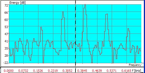
Figure 5‑12: Incorrect FFT-analysis due to a too big time window, resolution 1024 points
3. Step – Increase of the temporal resolution through decrease of the
FFT resolution
Following is to be done to
decrease the analysis time window (= decrease of the FFT-resolution):
One
- sets in the
window „Functions and parameters->Spektralanalysis” () in the
field frequency domain / Resolution the value 256 instead of 1024, the
Hann windowing keeps on existing,
- presses the key „Start" ,
- presses the
key „Automatic scaling” in the main window after finishing of the
spectrogram.
The result of the higher
time-resolution shows the next figure:
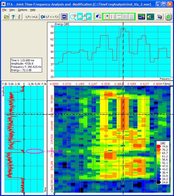
Figure 5‑13: FFT-analysis, FFT-resolution 256 points
One sees that now the
spectrogram begins to show more variations. The disposition to the smearing in
time direction decreases. Naturally the frequency uncertainty increases
correspondingly. Nevertheless the spectrogram still seems blurred especially in
the field of the upper signal block.
Now an experiment shall show
whether the detailed degree can be improved by a further increase of the
temporal resolution through decrease of the FFT-resolution.
4. Strep - Further increase of the temporal resolution through decrease
of the FFT resolution
E.g. the following is to be
done to arrange a further decrease of the analysis time window (= decrease of
the FFT-resolution):
One
- sets in the
window „Functions and parameters->Spektralanalysis” () in the
field frequency domain / Resolution the value 64 instead of 256, the Hann
windowing keeps on existing,
- presses the key „Start" ,
- presses the
key „Automatic scaling" in the main window after finishing of the
spectrogram.
The result of the higher
time-resolution shows the next figure.
It is to be observed:
- For the first time the signal pause between the
two signal blocks is to be recognized also clearly in the spectrogram.
- In the area of the upper signal block the
smearing in time direction decreased so far that finally no continuous
frequency allocations are indicated anymore.
Important: If the 5 dominant
frequency components indicated in former figure would actually exist in the
signal, they would keep on being preserved also after the further decrease of
the FFT-resolution in the spectrogram. Maybe this statement should be
considered shortly and comprehended because it is part of the
parameterization strategy.
- The uncertainty in frequency direction increased again:
![]()
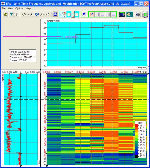
Figure 5‑14: FFT-analysis, FFT-resolution 64 points
Obviously for the temporal
resolution of the signal an analysis time window of 64 samples (=> FFT
resolution 64 points) is a good provisional value for a DXP analysis. Then not
only the temporal- but also the frequency resolution will increase again.
That happens in the next
step:
5. Step – Increase of the
measurement accuracy in time- and frequency-direction with DXP
In the former sections it was
to be recognized that an analysis time interval of 64 samples is to be preferred
to a value by 256 at least.
- Therefore an analysis time interval of 64 samples
shall serve as a start value for the DXP-analysis.
- Since DXP is only reasonable if the frequency
domain resolution is bigger than the analysis time interval, a value is
immediately applied by 2048.
In order to carry out the
transformation correspondingly the following is to do:
One
- sets in the
window „Functions and parameters->Spektralanalysis” () the
transformation method to „DXP-I" with a frequency domain resolution
of 2048 as well as Hann windowing,
- sets up the
value 64 as well as also Hann-windowing in the same window in the field
“time domain”,
- presses the key „Start" ,
- presses the
key „Automatic scaling" in the main window after finishing of the
spectrogram.
The result of the
DXP-transformation is to be seen in the next figure. One pays attention to:
- The uncertainty area has changed from
 to
to  what is achieved through the increase of
the frequency resolution through DXP.
what is achieved through the increase of
the frequency resolution through DXP. - For the first time a FSK-typical spectrogram
arises which represents the instantaneous frequency course.
The indicated time interval
is, however, much too big in order to be able to align the FSK-signal. This may
be easily changed through a temporal zoom.
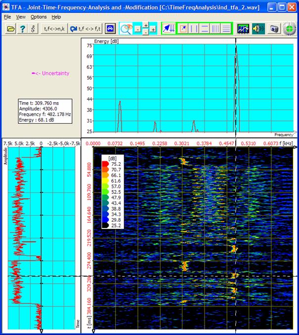
Figure 5‑15: DXP-I-analysis, resolution 2048 points, time interval 64 samples
The upper signal block mainly
contains a so-called REVs- sequence and therefore it may be not very
interesting. Arbitrary the lower block is selected for the further measurement.
That happens in the next step:
6. Step - In-Zoom into an
interesting time signal section
Now it shall be demonstrated
how a mouse-supported time interval zoom can be done, keyword „Area selection” ![]() according to section 4.3.7 with drawing a selection rectangle in the time domain
or in the time-frequency domain and after that performing a zoom.
according to section 4.3.7 with drawing a selection rectangle in the time domain
or in the time-frequency domain and after that performing a zoom.
The following is to be done:
One
- presses the key , in order to
obtain the area selection mode,
- draws in the time domain with the mouse a
selection rectangle around the lower signal block, for instance as
follows:
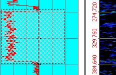
- presses the upper -key in the
main program window, to arrange a vertical zoom into the marked area.
The following figure shows
the result:
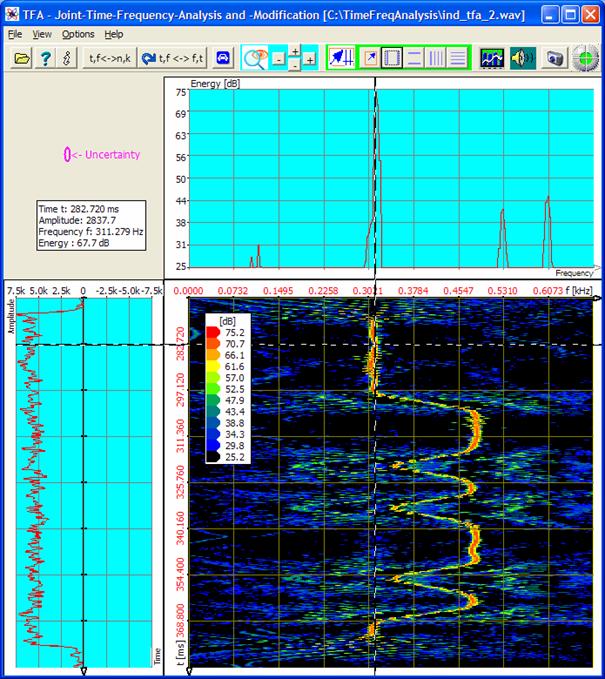
Figure 5‑16: DXP-I-analysis, resolution 2048 points, time interval 64 samples
Now one can recognize the FSK-signal sufficiently well for a
measurement.
7. Step - Signal measurement
According to the task the two
shift frequencies and the modulation rate are to be measured. To that are used:
- „Vertical markers" according to section 4.3.8
- „Horizontal Harmonic-markers” according to
section 4.3.11
The following is to be done:
One
- presses the keys and
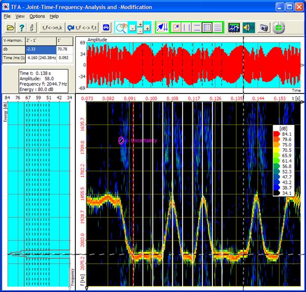 for the activation the vertical markers
and the horizontal Harmonic markers,
for the activation the vertical markers
and the horizontal Harmonic markers, - moves the markers with the mouse pointer onto the
positions to be indicated,
- reads off the measured values, either directly in
the main window’s maker value table or after pressing of the main window
key
 in the window „Functions and parameters
->XY-Markers”:
in the window „Functions and parameters
->XY-Markers”:
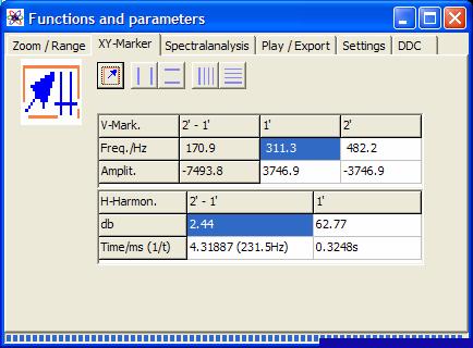
Figure 5‑17: The results given by the marker value table
Result:
- The shift frequency is 170,9 Hz.
- The modulation rate is 231,5 Bd.
Of course the result accuracy
can be increased by a better choice of the zoom-intervals furthermore.
The following figure shows an
example for positioning the markers for the signal measurement:
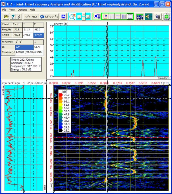
Figure
5‑18: Signal measurement
5.2
Filtering
A precise time-frequency
analysis simplifies the
signal
filtering and signal extraction too. With the already in section 5.1 used signals that shall be demonstrated in the
following.
5.2.1
Speech
signal: Extraction of the F0-oscillation
In section 5.1.1 the F0-frequency was measured at a certain moment.
Now the point is, to extract this oscillation and to open a new TFA program
instance with it.
To that one can run through e.g. following steps:
1. Step – Opening the file and representing it clearly
One
- opens the
file „ind_tfa.wav" ,
- marks all
view-options,
- sets in the
window „Functions and parameters->Spektralanalysis” () the
transformation method to „FFT" with a resolution 1024,
- presses the key „Start" ,
- presses the
key „Automatic scaling" in the main window,
- presses possibly
the keys „Presentation continuously / discrete" and/or „Orientation" .
It will appear the already
shown program window Figure 5‑5, that is placed here once more. According to the PC
system the figure can differ a bit, and of course e.g. the XY marker depends on
the position of the mouse pointer, and so forth.
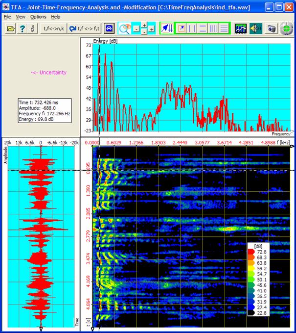
Figure 5‑19: File „ind_tfa.wav“, FFT-analysis, resolution 1024 points
From section 5.1.1 it is known that the F0-frequency was near about 180
Hz. In order to be able to recognize this frequency range better, a frequency-zoom
according to section 4.3.13 „Zoom“ e.g. into the area 0...600 Hz may be helpful. That
happens in the next step.
2. Step - Frequency-zoom
For that there are several possibilities:
- Direct
specification of the indicated area via the key , cf. section
4.3.14 “Advanced zoom/boundary function"
- Area
selection according to section 4.3.7 and zoom
- Use of the
„vertical markers" and the „horizontal markers" according to sections 4.3.8 and 4.3.9
This time the first method is shall be used. To carry out the zoom the
following is to do:
- One presses the key , the window
„Functions and parameters-> Zoom/Range" appears:
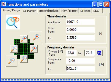
Figure 5‑20: Operation window „Functions and parameters ->Zoom / Range“
- One enters the frequency range of 0...600 Hz,
whereon the following program main window appears:

Figure 5‑21: Frequency-zoom, FFT-analysis, resolution 1024 points
With this FFT-setting the
uncertainty in frequency direction ![]() is still quite large. That complicates the
choice of a suitable frequency section for the extraction.
is still quite large. That complicates the
choice of a suitable frequency section for the extraction.
3. Step – Increase of the frequency resolution under retention of the
temporal resolution
This is possible only with the DXP-transformation method. A first
approach is the choice of
- frequency
resolution as 4096 points and of the
- analysis time
window size as 1024 samples.
In order to carry out the transformation correspondingly the following
is to do. One
- sets in the
window „Functions and parameters->Spektralanalysis” () the
transformation method to „DXP-I" with a frequency resolution of 4096
as well as Hann windowing,
- sets the time
interval in the filed “time domain” to the value 1024 and again “Hann” as
a window function,
- presses the key „Start" ,
- presses the
key „Automatic scaling" in the main window after finishing of the
spectrogram.
The result of the
DXP-transformation is to be seen in the next figure.
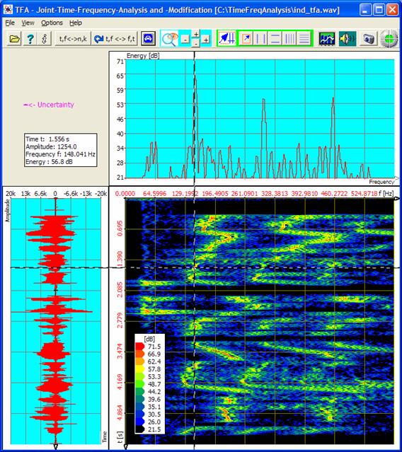
Figure 5‑22: DXP-I-analysis, resolution 4096 points, time interval 1024 samples
The result is still a little blurred, which has to do with the still
quite big analysis time window. Therefore an analysis time window of 256
samples instead of 1024 samples alike section 5.1.1 is used next. That shows following representation:
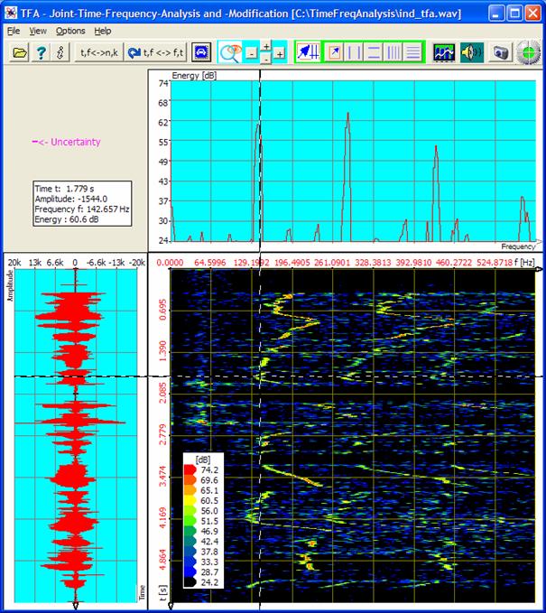
Figure 5‑23: DXP-I-analysis, resolution 4096 points, time interval 256 samples
The F0-area is to be
estimated quite good now and can be marked, without getting in contact with too
many other signal parts. That happens in the next step:
4. Step - Extraction of the F0-area
The marking of the F0-area
shall be carried out freehand via the area selection ![]() according to section.4.3.7.
according to section.4.3.7.
The
following is to be done:
One
- presses the key , in order to
enter the area selection mode,
- draws a selection rectangle in the time-frequency
domain with the mouse around the area that is occupied by F0 - if
possible, without marking the neighbouring harmonic:
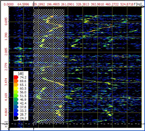
- presses the key
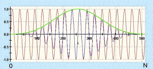 , to open the
operation window „Functions and parameters" directly at the register
tab „Play / export",
, to open the
operation window „Functions and parameters" directly at the register
tab „Play / export", - presses the key
 , in order to
open a new TFA instance,
therefore a new TFA program window that only
indicates the selected signal. Notice: This process may take some time.
Possibilities of the acceleration are to be found in section 4.3.16.
, in order to
open a new TFA instance,
therefore a new TFA program window that only
indicates the selected signal. Notice: This process may take some time.
Possibilities of the acceleration are to be found in section 4.3.16.
The following figure shows
the result:
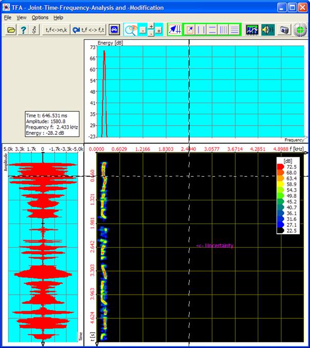
Figure 5‑24: DXP-I-Extraction at an resolution of 4096 points, time interval 256 samples
The extracted new signal
contains only still the F0-frequency portions. As shown in this documentation
it can be analyzed more extensively.
5.2.2
Communication
engineering: Extraction of a FSK-signal
In section 5.1.2 the modulation parameters of a FSK-signal were
analyzed. Now the point is, to extract an export a signal portion (here in the
example: the second signal block) specified temporal and in its frequency.
To this one can run through e.g. following steps:
1. Strep – Opening file open and representing it clearly
One
- opens the
file „ind_tfa_2.wav" ,
- marks all
view-options,
- sets in the
window „Functions and parameters->Spektralanalysis” () the
transformation method to „FFT" with a resolution of 1024,
- presses the key „Start" ,
- presses the
key „Automatic scaling" in the main window,
- presses
possibly the keys „Presentation continuously / discrete" and/or „Orientation" .
The in section 5.1.2 shown program window will appear that is placed here
again. According to the PC system the figure can differ a bit, and of course
e.g. the XY marker depends on the position of the mouse pointer, and so forth.
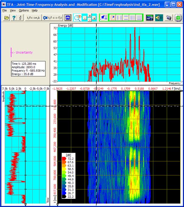
Figure 5‑25: File „ind_tfa_2.wav“, FFT-analysis, resolution 1024 points
Obviously the signal section
contains 4 signal blocks, of which each two are nearby.
The objective of this
exercise is to extract and export the second signal block temporal and within
its frequency range.
For this purpose it is at
first useful to represent the block sharply. That happens in the next step.
2. Step - Precise representation of the signal block to be exported
Section 5.1.2 showed that the DXP-I-Analyse with a frequency
resolution of 2048 points and an analysis time window of 64 samples provides a
quite sharp representation of the signal.
In order to display the
signal block to be exported, the following is to be done:
One
- carries on the steps according to section 5.1.2 up to and including step 5 again,
- presses the key , in order to
enter area selection mode,
- draws a selection rectangle in the time-frequency
domain with the mouse around the second signal block:
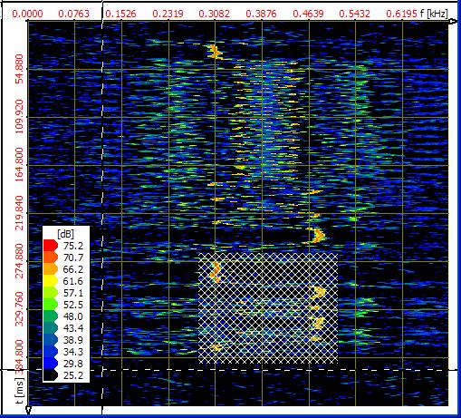
- presses the key , to open the
operation window „Functions and parameters" directly with the register
tab „Play / export",
- presses the key
 , the output
of the selected signal is carried out via a WAV-“Saving file as…
"-dialog. Notice: This process may take some time. Possibilities for
an acceleration are to be found in section 4.3.16.
, the output
of the selected signal is carried out via a WAV-“Saving file as…
"-dialog. Notice: This process may take some time. Possibilities for
an acceleration are to be found in section 4.3.16.
5.3
Frequency conversion
The means of the TFA
time-frequency analysis also simplify the frequency conversion and the extraction of
signal portions. Using the signals known already from the former exercises this
shall be demonstrated in the following.
5.3.1
Speech
signal: Making audible a discant voice component
In this section a higher
frequency band outside of the hearing distance shall be
- displaced into a lower-frequency region (frequency
conversion)
- exported as a file
and
- played back via the loudspeakers.
These three points are now
handled in separate sections.
5.3.1.1 Frequency
conversion
For this one can run through e.g. the following steps:
1. Step – Opening file and representing it clearly
One
- opens the
file „ind_tfa.wav" ,
- marks all
view-options,
- sets in the
window „Functions and parameters->Spektralanalysis” () the
transformation method to „FFT" with a resolution of 1024,
- presses the key „Start" ,
- presses the
key „Automatic scaling" in the main window,
- presses
possibly the keys „Presentation continuously / discrete" and/or „Orientation" .
It will appear the program
window that is already known from Figure 5-5. It is placed here again. According to the PC system
the figure can differ a bit, and of course e.g. the XY marker depends on the
position of the mouse pointer, and so forth.


Figure 5‑26: File „ind_tfa.wav“, FFT-analysis, resolution 1024 points
The arbitrarily chosen task
insists on shifting the in white encircled time-frequency area to the left
nearby the zero frequency position. One estimates briefly that it is a matter
of about 2 seconds of length and a frequency range of around about 2 kHz.
For the selection of a time-frequency
area there are the methods described in the sections 4.3.7 “Area selection" up to 4.3.9 “Horizontal marker„. Here the freehand marking of the area shall be
carried out via the area selection ![]() according to section 4.3.7. The following is to be done:
according to section 4.3.7. The following is to be done:
2. Step - Area selection and DDC
One
- presses the key , in order to
enter the area selection mode,
- draws a selection rectangle in the time-frequency
domain with the mouse for instance around the area marked through the
white circle:
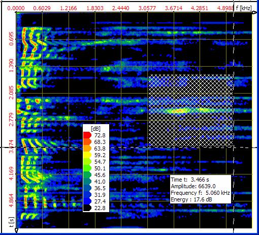
- presses the key , in order to
open the operation window „Functions and parameters",
- chooses the register tab „DDC"
 , whereupon
the DDC control panel appears:
, whereupon
the DDC control panel appears:
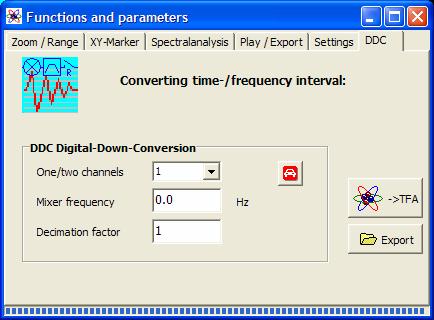
Figure 5‑27: Operation window „Functions and parameters -> DDC“
- presses the key
 , to obtain a
proposal for the DDC settings:
, to obtain a
proposal for the DDC settings:
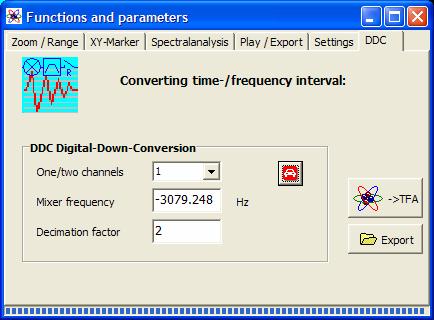
Figure 5‑28: DDC-setting proposal for real-valued frequency conversion
Notice How does TFA
amount these setting values?
- One/two channel file: Since the chosen audio
file has 1 channel, TFA acts on the assumption of „One/two channel
file = 1".
- Mixer frequency: Since for instance the
lower limiting frequency of the area selection is near 3 kHz, that is the
shift in the direction of the zero frequency position which does not lead
to a transgression of the boundary f=0 yet.
- Decimation factor: Since the width of the
selected frequency band is about 2 kHz, the sampling rate may be halved
through „Decimation factor = 2".
The frequency conversion
takes place in the course of the file export or at handover onto a new TFA-instance.
5.3.1.2 File export
![]()
For the file export this key
is to be pressed. A usual “File-save-as…”-dialog leads through the further
steps. The file export can happen as a WAV file for the signal exchange to
other applications or as a 32-bit TFA file together with further information,
e.g. the starttime of the interval.
5.3.1.3 TFA
instance
![]()
In order to open a new TFA instance, therefore a new TFA program window that indicates only the selected signal, this key
is to be pressed. After pressing of „Automatic scaling" ![]() the new TFA instance is shown like as follows.
Attention is to be paid to the frequency resolution that is not 1024 but 4096.
the new TFA instance is shown like as follows.
Attention is to be paid to the frequency resolution that is not 1024 but 4096.
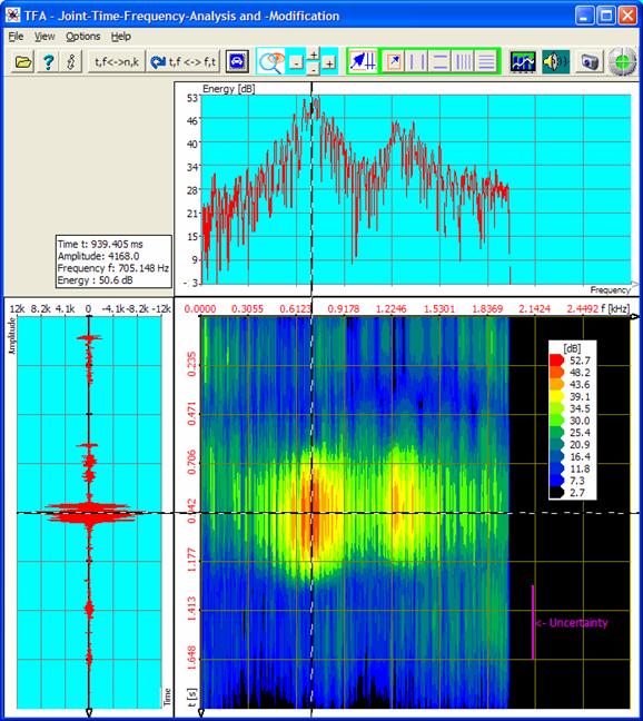
Figure 5‑29: New TFA instance with the frequency converted and decimated signal
In order to play back e.g.
the entire area via speakers, one
- marks e.g. the entire time interval in the time
window to the left, while the selection mode is activated,
- pushes the icon for opening the operation window
„Functions and parameters" directly with the register tab "Play
/ export" and
- uses the keys in usual manner
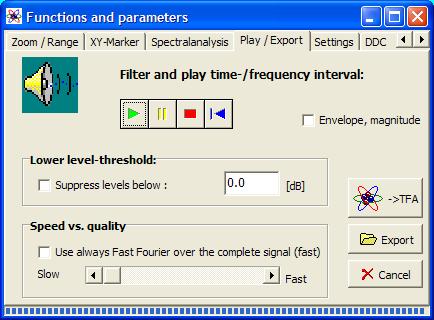 .
.
The playback of signal
intervals is detailed described in section 4.3.16 “Play / Export".
5.3.2
Communication
engineering: Conversion of a real-valued signal into the complex base band
In section 5.1.2 it was to be seen that the signal sample „ind_tfa_2.wav"
in fact represents a modulation signal from the communication engineering. It
is given in an intermediate frequency band (ZF, IF), what makes possible the
real-valued (one channel) storage.
For many methods of analysis,
as e.g. the instantaneous value analysis, the complex baseband instead of the
intermediate frequency band is more favourable. This requires the
complex-valued (two channel) signal storage since in this case in addition to
the so-called real part there is the so-called imaginary part.
The transformation of a real
signal or complex valued signal section (like in this case) into a complex signal
is object of this section.
For this one can run through e.g. following steps:
1. Step – Opening file and representing it clearly
One
- opens the
file „ind_tfa_2.wav " ,
- marks all
view-options,
- sets in the
window „Functions and parameters->Spektralanalysis” () the
transformation method to „FFT" with a resolution of 1024,
- presses the key „Start" ,
- presses the
key „Automatic scaling" in the main window ,
- presses
possibly the keys „Presentation continuously / discrete" and/or the key „Orientation" .
It will appear the program
window shown in section 5.1.2 that is here placed again. According to the PC system
the figure may differ a bit and of course e.g. the XY marker depends on the
position of the mouse pointer, and so forth.
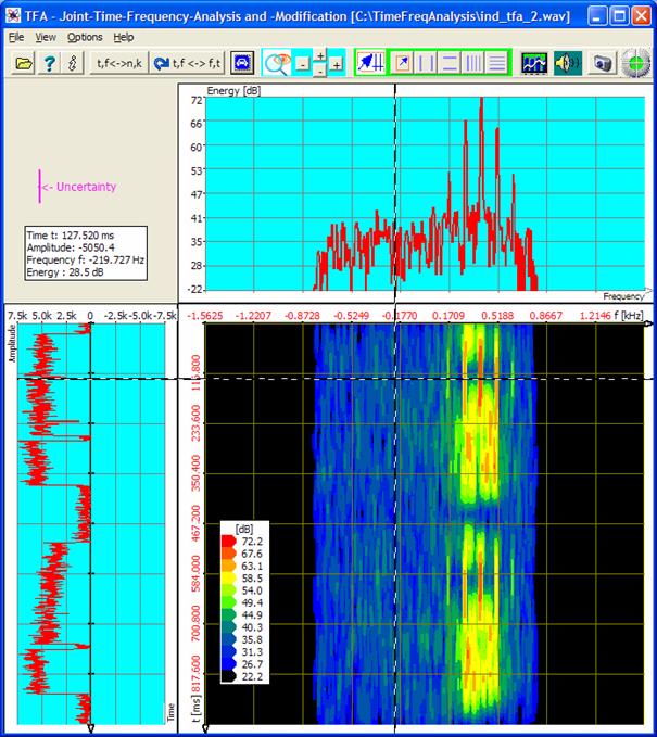
Figure 5‑30: File „ind_tfa_2.wav“, FFT-analysis, resolution 1024 points
The center frequency is about
f=390 Hz. The bandwidth, that show the vertical markers, is about BB
= 800 Hz, cf. following figure:
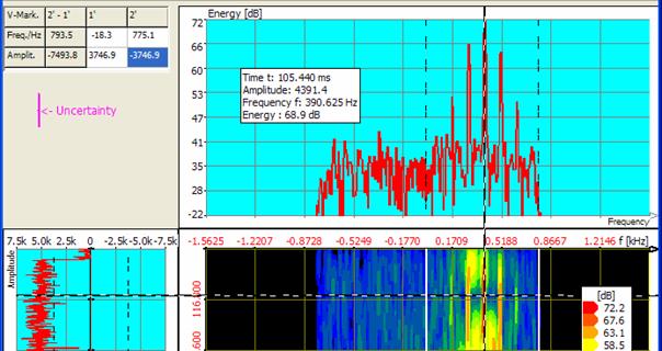
Figure 5‑31: Center frequency and bandwidth of a communicatin signal
That with the vertical marker
enclosed frequency band is now to be mixed to the left into the zero frequency
position that the center frequency coincides with the frequency of f=0.
2. Step - Area selection and DDC
- If the positioning of the vertical markers took
place in the spectrum (upper window), the signal is thus selected, which
means that a signal modification affects the entire signal within a given
time. The area selection is thus already carried out.
- One presses the key , in order to
open the operation window "Functions and parameters".
- One chooses the register tab „DDC" , whereupon
the DDC control panel appears, and presses the key , to obtain a
proposal for the DDC settings:
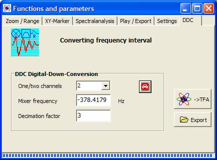
Figure 5‑32: DDC-setting proposal for complex baseband
Notice How does TFA
amount these setting values?
- One/two channel file: Since the chosen
audio file has two channels TFA acts on the assumption of „One/two
channel file = 2".
- Mixer frequency: Since for instance the center frequency
of the area selection is near 378 Hz, that is the shift in the direction
of the zero frequency position balanced to f=0.
- Decimation factor: Since the width of the
selected frequency band is about 800 Hz, the sampling rate may be halved
through „Decimation factor = 3".
The frequency conversion
takes place in the course of the file export or at handover onto a new TFA-instance.
5.3.2.1 File export
![]()
For the file export this key
is to be pressed. A usual “File-save-as…”-dialog leads through the further
steps. The file export can happen as a WAV file for the signal exchange to
other applications or as a 32-bit TFA file together with further information
like the starttime of the interval.
5.3.2.2 New TFA instance with DDC-result
![]()
In order to open a new TFA instance, therefore a new TFA program window that indicates only the selected signal, this key
is to be pressed. After pressing of „Automatic scaling" ![]() the new TFA instance is shown like as follows:
the new TFA instance is shown like as follows:
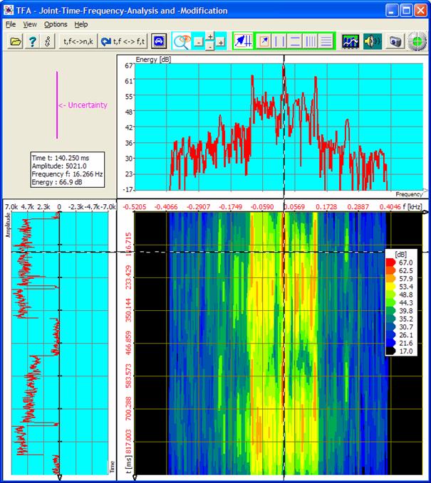
Figure 5‑33: New TFA-Instanz with a signal in the complex baseband
At the beginning it was
found, that the center frequency lay at about f=390 Hz. In the figure
above it can be read off that now after frequency conversion it is near about 16
Hz. That means, that a value of -390 Hz as the “Mixer frequency” in the DDC
control panel would have centred the signal better.
5.4
Analysis
of Modulation spectra
The characteristic sound of
e.g. music instruments or the human speech also comes from the modulation of
the included frequency components. They are responsible for a sounds liveliness
and allow us, e.g. to distinguish different violin fabricats or speekers.
This section gives an example
for possible steps of an modulation spectra analysis based on a sample of a
singing bowl (in german called “Klangschale”):
- Selection and extraction of a frequency component
as its envelope
- Analysis of the modulation spectrum
At this place sincere thanks
are given to the company „Synotec Psychoinformatik GmbH, Geyer“ for the
retrieval of the signal “Klangschale.wav” that ist included in TFAs samples.
5.4.1
Selection
and extraction of a frequency component as its envelope
To do this on may perform the
following steps:
1. Step – Assure, that the option “DC-Offset-Correction” is set
With regard to the later calculation of the signals envelope and its
spectrum this is not necessary but advantageous it TFA doesn’t start with this option set right from start.
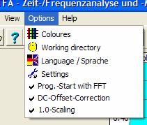
The reason is, that the magnitude always includes a mostly uniteressting
DC-Offset which may lead to a dominate spectral line at the frequency 0 Hz
without informative value. This may compromise the automatic scaling ![]() , because it has to regard the 0-Hz-Peak.
, because it has to regard the 0-Hz-Peak.
If the option is not set, one should do this, then close TFA and start again. When the program
is closed many settings like the “DC-Offset-Correction”
are saved and do not need to be controlled after a new start.
2. Step – Open wav-file and present it clearly
arranged
One
- opens the file “Klangschale.wav”
- marks all view
options
- sets in the
window „Functions and parameters->Spektralanalysis” () the
transformation method to „FFT" with a resolution of 8192,
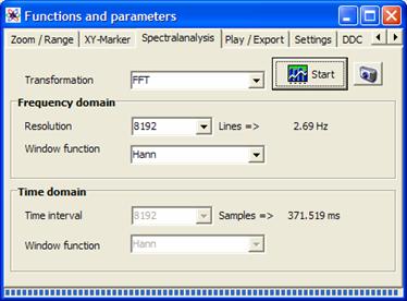
- presses the key „Start" ,
- presses the
key „Automatic scaling" in the main window ,
- presses possibly
the keys „Presentation continuously / discrete" and/or the key „Orientation" .
It will appear the following program
window. According to the PC system the figure may differ a bit and of course
e.g. the XY marker depends on the position of the mouse pointer, and so forth.
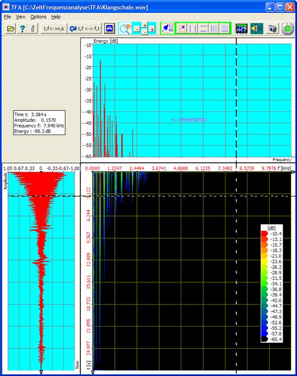
Figure 5‑34: TFA after opening the signal “Klangschale.wav”
The signals energie is mainly located in the frequency range up to about
4 kHz. A first zoom enhances the overview.
One
- presses the button to enter the area selection mode
- draw a
selection area rectangle in the frequency domain to mark the main energy
range,
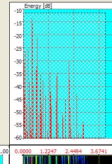
- presses
the right button
 in the field
  to perform a horicontal zoom in frequency
direction,
to perform a horicontal zoom in frequency
direction, - presses the button “Automatic Scaling” what may
enhance the view.
Now the program window should look like:
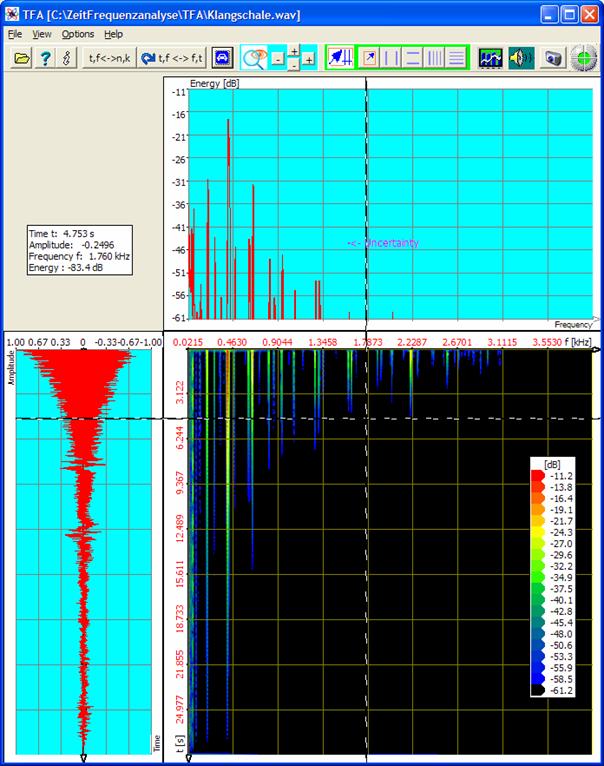
Figure 5‑35: Zoom in frequency range
No the spectrum of the singing bowl is more considerable.
In the following the arbitrary goal is setted to obtain the modulation
spectrum of the red coloured overtone and therefore to mark and to export its
magnitude signal.
3. Step – Marking the frequency componet and exporting the magnitude
signal
The marking of the frequency component again my be done like shown above
or
- with the
vertical markers
 ,
, - that can be moved freehand or via entering the
exact positions in the table (please regard the units).
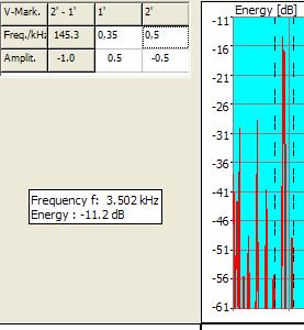
Now the frequency range 350 Hz to 500 Hz is selected.
Of course the selection can also be done in the time-/frequency domain.
- One presses nun the button to open the in the window „Functions and
parameters“.
- One chooses the card „DDC“ , the
DDC-control panel appears. Press the button to obtain
a settings recommendation:
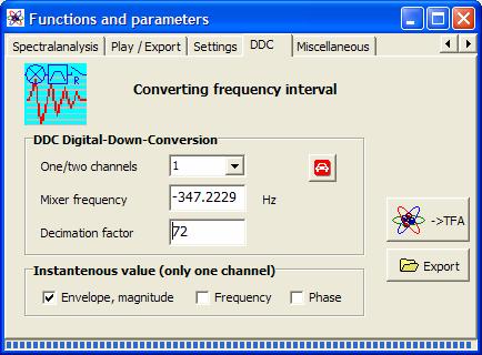
Figure 5‑36: DDC settings recommendation
Note: How does TFA calculate
this settings?
- One/two
channels: Because the given wave-file is a 1-channel-file TFA will propose this.
- Mixer frequency: Because the lower cut-off frequency of the
selected range is about 347 Hz, this is the shift towards the Zero-pitch f=0.
- Decimation factor: The upper cut-off frequency of the selected
range is about 500 Hz, die lower at about 350 Hz. So the frequency band
is about 150 Hz wide and the minimum sampling rate is 300 Hz. The actual
sampling rate is 22 kHz, that leads to a rounded decimation factor of 72.
- Check the field
 because not the signal
but its envelope shall be examinded.
because not the signal
but its envelope shall be examinded.
The frequency conversation is performed with the file export ort the
handover to a new TFA-Instance. The
last shall now be shown.
File export (not relevant for
next explanations)
![]()
In order to perform a file export this button is to be pressed. A common
“Save as...“-dialogue leads to the further steps. A file export can be done as
WAV-file for the exchange with other applications or as 32-Bit-TFA-file
together with other information, e.g. the starttime of a signal interval.
New TFA-Instance showing the
DDC-result
![]()
To open an new TFA-Instance, then a new TFA-program window, that shows only the
selected signal, this button is to be pressed. After pressing the button
“automatic scaling” ![]() the new TFA-Instance looks like the next but one figure:
the new TFA-Instance looks like the next but one figure:
If there are major differences probably the reason is the setting of the
FFT-resolution, see settings window:
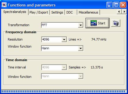
Figure 5‑37: FFT setting
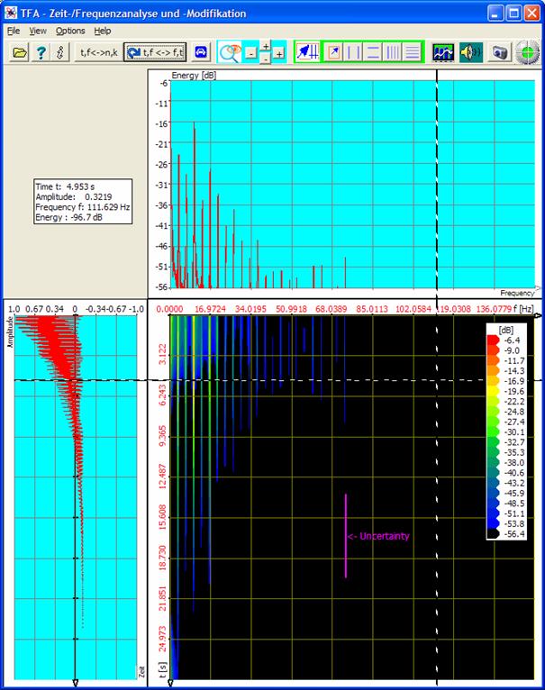
Figure 5‑38: Modulations spectrum of the selected overtone
Note:
Because of setting the DC-Offset-Option one sees a magnitude signal
without DC-offset. So there are negative values too.
Then
5.4.2
Analysis
of the modulation spectrum
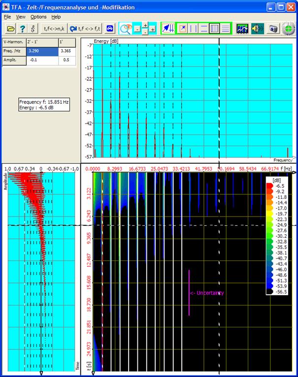
6
FAQ
– Frequenzly asked questions
This section answers
questions to TFA which came up by the time. According to version of this
text the list is not very long yet.
6.1
Uncoupling
XY-Marker and mouse pointer
Question: How can I achieve
that the XY-marker stands still and does not follow the mouse pointer?
Answer: If the TFA program window is active one presses the <Strg>-Taste. Then
only the mouse coordinates are changed in case of mouse pointer movement, the
XY marker stands still.
6.2
Long
duration of DXP-I-computation
Question: During the start
of the DXP-I-computation with a high frequency resolution it takes many seconds
until the first lines are drawn.
Answer: During the change
to the DXP-I-transformation method or change of the DXP- settings first of all
it is carried out the computation of a matrix. At this time the red status lamp
glows and the software does not seem to react. One waits this time span, after
that the reaction time is nearly zero.
6.3
View elements unvisible
Question: Although the view
element „uncertainty area" is visibly marked, is not to be seen in the
program window.
Answer: The view elements
can be moved with the mouse pointer in the area of the program window. It can
happen, that they screen themselves. That also happens, when the marker and so
that the marker value tables are turned on. Also they can screen view elements,
when latter are in the table area. One deactivates markers and view elements
and places the elements so that they do not collide. The „uncertainty
area" can be placed to its origin position by switching it off and on
again.
6.4
Unsatisfactory spectral resolution
Question: Using the
spectral transformation method DXP-I my with a sampling rate of 10 MHz recorded
measurement signal cannot be spectrally analyzed fine enough because, there is
a maximum resolution of only 4096 lines, what leads to a line mode separation
of more than 2441 Hz.
Answer: In DXP the
maximum frequency resolution is restricted to the value 4096, because higher
values would provoke a quadratic increasing of the computing duration and also
a higher memory requirement. There are, however, two ways out:
- Use of the transformation method FFT with however
the disadvantage of larger uncertainty
- Use of the transformation method DXP and use of
the Digital Down Converter (DDC) according to section 4.3.17 for the selection of interesting signal sections
of smaller frequency interval width. The increase of the Measurement
accuracy corresponds to the chosen DDC decimation factor.
6.5
Staircase-shaped
time signal after DDC-decimation
Question: After the use of
the DDC with reduction of the sampling rate the time signal appears rough and
staircase-shaped.
Answer: Even if the DDC
decimation factor is correctly adjusted so that the sampling rate at least
corresponds to the double of the highest signal frequency according to the
sampling theorem nevertheless that means that the highest frequency components
show only few samples per period. Curves can be represented no more. If this is
essential, however, one simply reduces the DDC decimation factor.
6.6
Installation
on a network drive
Question: Is it possible to
install TFA on a network drive?
Answer: Yes, but the
network drive must be addressable via a drive letter comparable to local drives.
Apart from this it is to be considered that if several persons use the software
simulanously the functions Playback and DDC are only constricted available.
7
Abbreviations
ARQ Block
transfer technique of the telecommunication engineering
ASK Radio
transmission technique, Amplitude-Shift-Keying
DDC Digital-Down-Converter
DFT Discrete
Fourier Transformation
FFT Fast
Fourier Transformation
FSK Radio transmission technique,
Frequency-Shift-Keying
HF High
frequency
IF Intermediate
frequency (IF): The intermediate frequency band is
the result from
down-converting e.g. a radio frequency band.
JTFA Joint-Time-Frequency
Analysis
LPC Linear
Predictive Coding,
NF Low
frequency
PSK Radio
transmission technique, Phase-Shift-Keying
REVs-Folge Reversal-Folge, 0101…-Bitsequence
TFA Time-Frequency
Analysis
USB Universal
Serial Bus
ZF German
for “IF”: Intermediate frequency (IF): The
intermediate
frequency band is the result from
down-converting
e.g. a radio
frequency band.
8
Table of figures
Figure 1‑1:
Speech sample, transformation FFT, FFT-length 4096
Figure 1‑2:
Speech sample, transformation FFT, FFT-length 512
Figure 1‑3:
Speech sample, transformation DXP-I, FFT-length 4096, 512 samples
Figure 2‑1:
Possible directory structure for the program installation
Figure 4‑1:
The TFA programm window after program start
Figure 4‑2:
TFA after opening file „IND_TFA.Wav“, FFT-lenght: 1024
Figure 4‑3:
TFA with enlarged time-frequency representation
Figure 4‑4:
TFA with enlarged time representation
Figure 4‑5:
Uncertainty area at transformation FFT, FFT-length: 1024
Figure 4‑6:
Uncertainty area at transformation FFT, FFT-length: 4096
Figure 4‑7:
Uncertainty area at DXP-I, resolution: 4096, time-window: 256 Samples
Figure 4‑8:
Operation window „Functions and parameters->Settings “
Figure 4‑9: Exchange of Orientation
Figure 4‑10:
Area selection in the time-frequency domain
Figure 4‑11:
Value table for vertical markers
Figure 4‑12:
Measurement exampe with „Vertical harmonic markers“
Figure 4‑13:
Operation window „Functions and parameters->XY-Marker“
Figure 4‑14:
Operation window „Functions and parameters->Zoom / Range“
Figure 4‑15:
Operation window „Functions and parameters ->Spektralanalysis“
Figure 4‑16:
A possible window funkction for weighting a time interval
Figure 4‑17:
Expansion
of a time interval Z (above) onto N samples (below
Figure 4‑18:
Windowing of the expanded time interval at N Samples
Figure 4‑19:
Operation window „Functions and parameters ->Play / Export“
Figure 4‑20:
Operation window „Functions and parameters ->DDC“
Figure 5‑1:
File „ind_tfa.wav“, FFT-analysis, resolution 1024 Points
Figure 5‑2:
Positioning of horizontal and vertical markers
Figure 5‑3:
Zoom in the time-frequency domain
Figure 5‑4:
Uncertainty area at a 4096-Points-FFT
Figure 5‑5:
FFT-analysis, resolution 4096 points
Figure 5‑6:
DXP-I-analysis, resolution 4096 points, time interval 1024 samples
Figure 5‑7:
DXP-I-analysis, resolution 4096 points, time interval 256 samples
Figure 5‑8:
DXP-I-analysis, resolution 4096 points, time interval 256 samples, Zoom
Figure 5‑9:
DXP-II-analysis, resolution 4096 points, time interval 256 samples, Zoom
Figure 5‑10:
File „ind_tfa_2.wav“, FFT-analysis, resolution 1024 points
Figure 5‑11:
Representation after zoom, FFT-analysis, resolution 1024 points
Figure 5‑12:
Incorrect FFT-analysis due to a too big time window, resolution 1024 points
Figure 5‑13:
FFT-analysis, FFT-resolution 256 points
Figure 5‑14:
FFT-analysis, FFT-resolution 64 points
Figure 5‑15:
DXP-I-analysis, resolution 2048 points, time interval 64 samples
Figure 5‑16:
DXP-I-analysis, resolution 2048 points, time interval 64 samples
Figure 5‑17:
The results given by the marker value table
Figure 5‑18: Signal measurement
Figure 5‑19:
File „ind_tfa.wav“, FFT-analysis, resolution 1024 points
Figure 5‑20:
Operation window „Functions and parameters ->Zoom / Range“
Figure 5‑21:
Frequency-zoom, FFT-analysis, resolution 1024 points
Figure 5‑22:
DXP-I-analysis, resolution 4096 points, time interval 1024 samples
Figure 5‑23:
DXP-I-analysis, resolution 4096 points, time interval 256 samples
Figure 5‑24:
DXP-I-Extraction at an resolution of 4096 points, time interval 256 samples
Figure 5‑25:
File „ind_tfa_2.wav“, FFT-analysis, resolution 1024 points
Figure 5‑26:
File „ind_tfa.wav“, FFT-analysis, resolution 1024 points
Figure 5‑27:
Operation window „Functions and parameters -> DDC“
Figure 5‑28:
DDC-setting proposal for real-valued frequency conversion
Figure 5‑29:
New TFA instance with the frequency converted and decimated signal
Figure 5‑30:
File „ind_tfa_2.wav“, FFT-analysis, resolution 1024 points
Figure 5‑31:
Center frequency and bandwidth
of a communicatin signal
Figure 5‑32:
DDC-setting proposal for complex baseband
Figure 5‑33:
New TFA-Instanz with a signal in the complex baseband
Figure 5‑34:
TFA after opening the signal “Klangschale.wav”
Figure 5‑35:
Zoom in frequency range
Figure 5‑36:
DDC settings recommendation..
Figure 5‑38:
Modulations spectrum of the selected overtone
9 Annex
9.1 Layout of the TFA-File-Format
The TFA-format supports the following:
- Samples are
stored in the format 32-bit-Float instead of having
samples as 16-bit integer values. Through that in case of the
signal-export and/or signal-import the otherwise always occurring
conversion loss is dropped.
- The sampling
rate is also stored as 32-bit-Floating point, to support very slow
processes, (e.g. earth science) and also very fast ones (e.g. radio
technology).
- The format includes a timestamp, so that the time-reference does not get lost due to
signal extractions.
The layout of the
TFA-file-format is given as follow. It consists of:
- Header-Block including the above
mentioned parameters
- Sequence of the Samples
The Header-Block is defined as:
// Header-Block des TFA-Dateiformats
typedef struct TFAInfo_pattern_type
{
char
pcFormatKennung[20]; // Text:
"TFA-Format"
long
lBitzahl; // Bei TFA
immer 32 (32 Bit)
long
lKanalzahl; // 1: reelle Datei, 2: komplex
float
fSamplingrate; //
Abtastrate in Hz
long
lAbtastwertezahl; // Anzahl reeller o. komplexer Samples
long
lSkalaInJahren; // 1, für
geophysikalische Zwecke
float
fStartzeitoffset; // Das 0-te
Sample entstand zu
//
dieser Zeit
char
pcEinheitStringStart[10]; // Einheit
der Startzeit
char
pcEinheitStringSampl[10]; // Einheit
der Samplingrate
long lInstanznummer; // Wieviele TFA-Instanzen
aktiv?
char
pcZusatzinfo[100]; // Nicht
benutzt
float
fErsatzFloat1; //
Erstzwerte für Zukünftiges
float
fErsatzFloat2; // Nicht
benutzt
float fErsatzFloat3; // Nicht benutzt
long
lErsatzLong1; // Nicht
benutzt
long
lErsatzLong2; // Nicht
benutzt
long
lErsatzLong3; // Nicht
benutzt
} TFA_HeaderInfo_type;
After the Header-Block the
samples follow. In case of complex-valued files the sequence is Re[0], Im[0],
Re[1], Im[1], …. , Re[lAbtastwertezahl-1], Im[lAbtastwertezahl-1].
10
History
This section lists least changes of the software TFA and this
documentation:
30.07.2010 –
Version x.033
Software:
- Export of spectral-line-vectors as [dB]-values in
textfile
- New DXP-transformation-variant for even higher
precision
Dokumentation:
- Description of the software amendments
14.05.2010 –
Version x.031
Software:
- Amendment of the Play/Export-function with
optional instantaneous value export (envelope = magnitude) for modulations
spectra analysis
- Amendment of the DDC-function with optional
instantaneous value export (envelope = magnitude, frequency and phase)
Dokumentation:
- Description of the software amendments
- Exercise
course modulations spectra analysis
12.05.2010 –
Version x.031
Software:
- Calculaton of instantenous values like envelope/maginitude
e.g. for modulation spectra analysis
Documentation:
- Description of the software amendments
15.04.2010 – Version x.030
Software:
- New signal file formats for open, convertion,
export and saving: 24-Bit-PCM (1- and 2-channels), 32-Bit-PCM (1- and 2-channels)
und 24-Bit-FLOAT (1- and 2-channels)
- New
Option „1.0-scaling“
Documentation:
- Description of the software amendments
01.05.2009 –
Version x.018
Software:
- For a better support of applications of earths sciences
the frequency scale can be calculated as periodic time between
samples with the unit “year” [yr].
- The time scale now may include a start time
offset as the addition of the time stamp of the beginning of the recording.
- Implementation of a new key field for temporal
navigating along the time axis.
- Amendment of the textfile-format for presetting
the start time and the sampling rate respectively the periodic time in [yr].
Documentation:
- Amendment of a clause that covers the temporal
navigating along the time axis
- Annotation of the new text-file-format
19.01.2009 –
Version x.014
Software:
- Elimination scaling error with energy-measurement
(less important)
- Improvement of the indication of time and frequency measured values
in case of sampling rates up to the MHz-range (more important)
- Graphic representation of complex valued data (dual-channel mode
with real part and imaginary part) in the time domain now as instantaneous
absolute value
Documentation:
- Additional
practice section for the functions of the Digital-Down-Converter (DDC)
- This page is intentionally left blank -